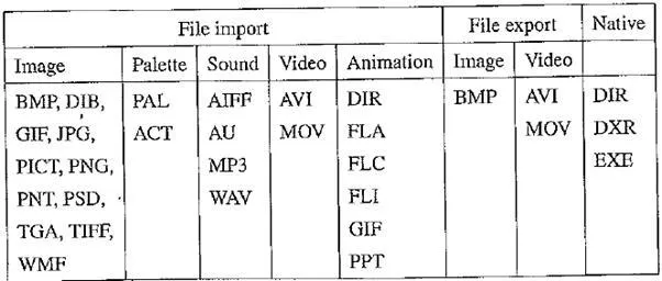
The number of file formats used in multimedia continues to proliferate. For example, the following table shows a list of file formats used in the popular product Macromedia Director. In this text, we shall study just a few popular file formats, to develop a sense of how they operate. We shall concentrate on GIF and JPG image file formats, since these two formats are distinguished by the fact that most web browsers can decompress and display them. To begin, we shall discuss the features of file formats in general.

Table Macromedia Director file formats

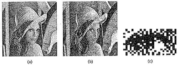
Monochrome 1 – bit Lena image

1 – Bit Images

Images consist of pixels, or pels— picture elements in digital images. A 1 – bit image consists of on and off bits only and thus is the simplest type of image. Each pixel is stored as a single bit (0 or 1). Hence, such an image is also referred to as a binary image.

It is also called a 1 – bit monochrome image, since it contains no color. The above figure shows a 1 – bit monochrome image (called “Lena” by multimedia scientists — this is a standard image used to illustrate many algorithms). A 640 x 480 monochrome image requires 38.4 kilobytes of storage (— 640 x 480 / 8). Monochrome 1 – bit images can be satisfactory for pictures containing only simple graphics and text.

8 – Bit Gray – Level Images

Now consider an 8 – bit image — that is, one for which each pixel has a gray value between 0 and 255. Each pixel is represented by a single byte — for example, a dark pixel might have a value of 10, and a bright one might be 230.

The entire image can be thought of as a two – dimensional array of pixel values. We refer to such an array as a bitmap, — a representation of the graphics / image data that parallels the manner in which it is stored in video memory.

Image resolution refers to the number of pixels in a digital image (higher resolution always yields better quality). Fairly high resolution for such an image might be 1,600 x 1,200, whereas lower resolution might be 640 x 480. Notice that here we are using an aspect ratio of 4:3. We don’t have to adopt this ratio, but it has been found to look natural.

Such an array must be stored in hardware; we call this hardware a frame buffer. Special (relatively expensive) hardware called a “video” card (actually a graphics card) is used for this purpose. The resolution of the video card does not have to match the desired resolution of the image, but if not enough video card memory is available, the data has to be shifted around in RAM for display.

We can think of the 8 – bit image as a set of 1 – bit bitplanes, where each plane consists of a 1 – bit representation of the image at higher and higher levels of “elevation”: a bit is turned on if the image pixel has a nonzero value at or above that bit level.

The following figure displays the concept of bitplanes graphically. Each bit – plane can have a value of 0 or 1 at each pixel but, together, all the bitplanes make up a single byte that stores values between 0 and 255 (in this 8 – bit situation). For the least significant bit, the bit value translates to 0 or 1 in the final numeric sum of the binary number. Positional arithmetic implies that for the next, second, bit each 0 or 1 makes a contribution of 0 or 2 to the final sum. The next bits stand for 0 or 4, 0 or 8, and so on, up to 0 or 128 for the most significant bit. Video cards can refresh bitplane data at video rate but, unlike RAM, do not hold the data well. Raster fields are refreshed at 60 cycles per second in North America.

Each pixel is usually stored as a byte (a value between 0 and 255), so a 640 x 480 grayscale image requires 300 kilobytes of storage (640 x 480 = 307,200).

If we wish to print such an image, things become more complex. Suppose we have a 600 dot – per – inch (dpi) laser printer. Such a device can usually only print a dot or not print it. However, a 600 x 600 image will be printed in a 1 – inch space and will thus not be very pleasing. Instead, dithering is used. The basic strategy of dithering is to trade intensity resolution for spatial resolution.

DitheringDithering is the most common means of reducing the color range of images down to the 256 (or fewer) colors seen in 8 – bit GIF images.

Dithering is the process of juxtaposing pixels of two colors to create the illusion that a third color is present. A simple example is an image with only black and white in the color palette. By combining black and white pixels in complex patterns a graphics program like Adobe Photoshop can create the illusion of gray values.

For printing on a 1 – bit printer, dithering is used to calculate larger patterns of dots, such that values from 0 to 255 correspond to pleasing patterns that correctly represent darker and brighter pixel values. The main strategy is to replace a pixel value by a larger pattern, say 2 x 2 or 4 x 4, such that the number of printed dots approximates the varying – sized disks of ink used in halftone printing. Half – tone printing is an analog process that uses smaller or larger filled circles of black ink to represent shading, for newspaper printing, say.

If instead we use an n x n matrix of on – off 1 – bit dots, we can represent n2 + 1 levels of intensity resolution — since, for example, three dots filled in any way counts as one intensity level. The dot patterns are created heuristically. For example, if we use a 2 x 2 “dither matrix”:

we can first remap image values in 0.. 255 into the new range 0.. 4 by (integer) dividing by 256/5. Then, for example, if the pixel value is 0, we print nothing in a 2 x 2 area of printer output. But if the pixel value is 4, we print all four dots. So the rule is

If the intensity is greater than the dither matrix entry, print an on dot at that entry location: replace each pixel by an nxn matrix of dots.

However, we notice that the number of levels is small for this type of printing. If we increase the number of effective intensity levels by increasing the dither matrix size, we also increase the size of the output image. This reduces the amount of detail in any small part of the image, effectively reducing the spatial resolution.

Note that the image size may be much larger for a dithered image, since replacing each pixel by a 4 x 4 array of dots, say, makes an image 16 times as large. However, a clever trick can get around this problem. Suppose we wish to use a larger, 4 x 4 dither matrix, such as

Then suppose we slide the dither matrix over the image four pixels in the horizontal and vertical directions at a time (where image values have been reduced to the range 0..16). An “ordered dither” consists of turning on the printer output bit for a pixel if the intensity level is greater than the particular matrix element just at that pixel position.

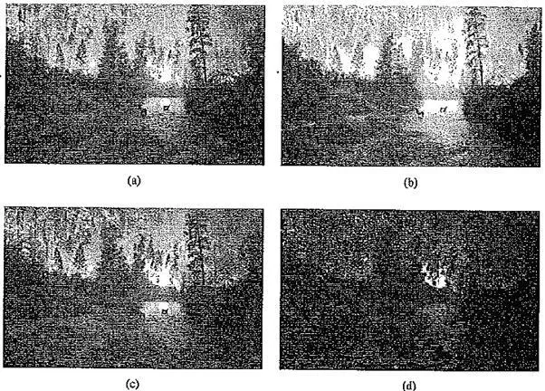
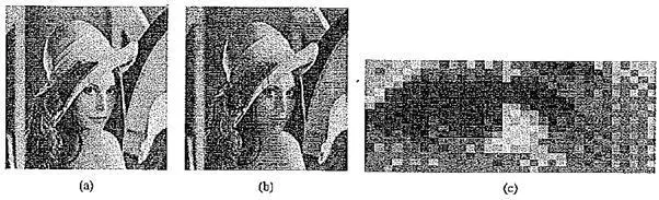
Dithering of grayscale images, (a) 8 – bit gray image lenagray.bmp; (b) dithered version of the image; (c) detail of dithered version. (This figure also appears in the color insert section.)

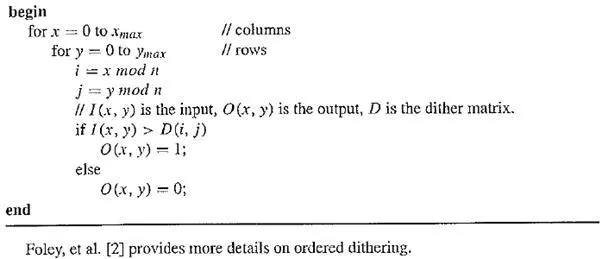
An algorithm for ordered dither, with n x n dither matrix, is as follows:

ALGORITHM ORDERED DITHER

Image Data Types

The next sections introduce some of the most common data types for graphics and image file formats: 24 – bit color and 8 – bit color. We then discuss file formats. Some formats are restricted to particular hardware / operating system platforms, while others are platform – independent, or cross – platform, formats. Even if some formats are not cross – platform, conversion applications can recognize and translate formats from one system to another.

Most image formats incorporate some variation of a compression technique due to the large storage size of image files. Compression techniques can be classified as either loss  less or lossy.

24 – Bit Color Images

In a color 24 – bit image, each pixel is represented by three bytes, usually representing RGB. Since each value is in the range 0 – 255, this format supports 256 x 256 x 256, or a total of 16,777,216, possible combined colors. However, such flexibility does result in a storage penalty: a 640 x 480 24 – bit color image would require 921.6 kilobytes of storage without any compression.

An important point to note is that many 24 – bit color images are actually stored as 32 – bit images, with the extra byte of data for each pixel storing an α (alpha) value representing special – effect information.

The above figure shows the image forest fire bmp, a 24 – bit image in Microsoft Windows BMP format (discussed later in the chapter). Also shown are the grayscale images for just the red, green, and blue channels, for this image. Taking the byte values 0..255 in each color channel to represent intensity, we can display a gray image for each color separately.

High – resolution color and separate R, G, B color channel images, (a) example of 24 – bit color image forest fire. bmp; (b, c, d) R, G, and B color channels for this image. (This figure also appears in the color insert section.)

8 – Bit Color Images

If space is a concern (and it almost always is), reasonably accurate color images can be obtained by quantizing the color information to collapse it. Many systems can make use of only 8 bits of color information (the so – called “256 colors”) in producing a screen image. Even if a system has the electronics to actually use 24 – bit information, backward compatibility demands that we understand 8 – bit color image files.

Such image files use the concept of a lookup table to store color information. Basically, the image stores not color but instead just a set of bytes, each of which is an index into a table with 3 – byte values that specify the color for a pixel with that lookup table index. In a way, it’s a bit like a paint – by – number children’s art set, with number 1 perhaps standing for orange, number 2 for green, and so on — there is no inherent pattern to the set of actual colors.

It makes sense to carefully choose just which colors to represent best in the image: if an image is mostly red sunset, it’s reasonable to represent red with precision and store only a few greens.

Suppose all the colors in a 24 – bit image were collected in a 256 x 256 x 256 set of cells, along with the count of how many pixels belong to each of these colors stored in that cell. For example, if exactly 23 pixels have RGB values (45, 200, 91) then store the value 23 in a three – dimensional array, at the element indexed by the index values [45, 200, 91]. This data structure is called a color histogram.

Three – dimensional histogram of RGB colors in forest fire .bmp

The above figure shows a 3D histogram of the RGB values of the pixels in forest fire.bmp. The histogram has 16 x 16 x 16 bins and shows the count in each bin in terms of intensity and pseudocolor. We can see a few important clusters of color information, corresponding to the reds, yellows, greens, and so on, of the forest fire image. Clustering in this way allows us to pick the most important 256 groups of color.

Basically, large populations in 3D histogram bins can be subjected to a split – and – merge algorithm to determine the “best” 256 colors.

Example of 8 – bit color image. (This figure also appears in the color insert section.)

This is not always the case. Consider the field of medical imaging: would you be satisfied with only a “reasonably accurate” image of your brain for potential laser surgery? Likely not —- and that is why consideration of 64 – bit imaging for medical applications is not out of the question. Note the great savings in space for 8 – bit images over 24 – bit ones: a 640 x 480 8 – bit color image requires only 300 kilobytes of storage, compared to 921.6 kilobytes for a color image (again, without any compression applied).

Color Lookup Tables (LUTs)

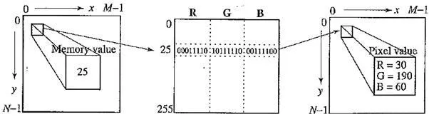
Again, the idea used in 8 – bit color images is to store only the index, or code value, for each pixel. Then, if a pixel stores, say, the value 25, the meaning is to go to row 25 in a color lookup table (LUT). While images are displayed as two – dimensional arrays of values, they are usually stored in row – column order as simply a long series of values. For an 8 – bit image, the image file can store in the file header information just what 8 – bit values for R, G, and B correspond to each index.

Color LUT for 8 – bit color images

Color picker for 8 – bit color: each block of the color picker corresponds to one row of the color LUT

A color picker consists of an array of fairly large blocks of color (or a semi – continuous range of colors) such that a mouse click will select the color indicated. In reality, a color picker displays the palette colors associated with index values from 0 to 255. The above figure displays the concept of a color picker: if the user selects the color block with index value 2, then the color meant is cyan, with RGB values (0, 255,255).

A simple animation process is possible via simply changing the color table: this is called color cycling or palette animation. Since updates from the color table are fast, this can result in a simple, pleasing effect.

Dithering can also be earned out for color printers, using 1 bit per color channel and spacing out the color with R, G, and B dots. Alternatively, if the printer or screen can print only a limited number of colors, say using 8 bits instead of 24, color can be made to seem printable, even if it is not available in the color LUT. The apparent color resolution of a display can be increased without reducing spatial resolution by averaging the intensities of neighboring pixels. Then it is possible to trick the eye into perceiving colors that are not available, because it carries out a spatial blending that can be put to good use.

How to Devise a Color Lookup Table?In general, clustering is an expensive and slow process. But we need to devise color LUTs somehow — how shall we accomplish this?

The most straightforward way to make 8 – bit lookup color out of 24 – bit color would be to divide the RGB cube into equal slices in each dimension. Then the centers of each of the resulting cubes would serve as the entries in the color LUT, while simply scaling the RGB ranges 0..255 into the appropriate ranges would generate the 8 – bit codes.

(a) 24 – bit color image lena.bmp; (b) version with color dithering; (c) detail of dithered version

Since humans are more sensitive to R and G than to B, we could shrink the R range and G range 0..255 into the 3 – bit range 0..7 and shrink the B range down to the 2 – bit range 0..3, making a total of 8 bits. To shrink R and G, we could simply divide the R or G byte value by (256/8 —) 32 and then truncate. Then each pixel in the image gets replaced by its 8 – bit index, and the color LUT serves to generate 24 – bit color.

However, what tends to happen with this simple scheme is that edge artifacts appear in the image. The reason is that if a slight change in RGB results in shifting to a new code, an edge appears, and this can be quite annoying perceptually.

A simple alternate solution for this color reduction problem called the median – cut algorithm does a better job (and several other competing methods do as well or better). This approach derives from computer graphics; here, we show a much simplified version. The method is a type of adaptive partitioning scheme that tries to put the most bits, the most discrimination power, where colors are most clustered.

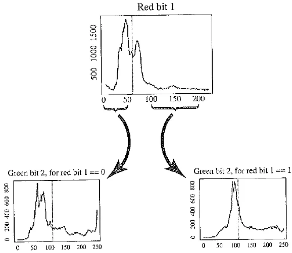
The idea is to sort the R byte values and find their median. Then values smaller than the median are labeled with a 0 bit and values larger than the median are labeled with a 1 bit. The median is the point where half the pixels are smaller and half are larger.

Suppose we are imaging some apples, and most pixels are reddish. Then the median R byte value might fall fairly high on the red 0.. 255 scale. Next, we consider only pixels with a 0 label from the first step and sort their G values. Again, we label image pixels with another bit, 0 for those less than the median in the greens and 1 for those greater. Now applying the same scheme to pixels that received a 1 bit for the red step, we have arrived at 2 – bit labeling for all pixels.

Carrying on to the blue channel, we have a 3 – bit scheme. Repeating all steps, R, G, and B, results in a 6 – bit scheme, and cycling through R and G once more results in 8 – bits. These bits form our 8 – bit color index value for pixels, and corresponding 24 – bit colors can be the centers of the resulting small color cubes.

You can see that in fact this type of scheme will indeed concentrate bits where they most need to differentiate between high populations of close colors. We can most easily visualize finding the median by using a histogram showing counts at position 0..255.

Histogram of Kbytes for the 24 – bit color image forest fire.bmp results in a 0 or 1 bit label for every pixel. For the second bit of the color table index being built, we take R values less than the R median and label just those pixels as 0 or 1 according as their G value is less or greater than the median of the G value. Continuing over R, G, B for 8 bits gives a color LUT 8 – bit index.

The 24 – bit color image resulting from replacing every pixel by its corresponding color LUT 24 – bit color is only an approximation to the original 24 – bit image, of course, but the above algorithm does a reasonable job of putting most discriminatory power where it is most needed — where small color shading differences will be most noticeable. It should also be mentioned that several methods exist for distributing the approximation errors from one pixel to the next. This has the effect of smoothing out problems in the 8 – bit approximation.

The more accurate version of the median – cut algorithm proceeds via the following steps:

1.      Find the smallest box that contains all the colors in the image.

2.      Sort the enclosed colors along the longest dimension of the box.

3.      Split the box into two regions at the median of the sorted list.

4.      Repeat the above process in steps (2) and (3) until the original color space has been divided into, say, 256 regions.

5.      For every box, call the mean of R, G, and B in that box the representative (the center) color for the box.

6.      Based on the Euclidean distance between a pixel RGB value and the box centers, assign every pixel to one of the representative colors. Replace the pixel by the code in a lookup table that indexes representative colors (in the table, each representative color is 24 – bits — 8 – bits each for R, G, and B.J

This way, we might have a table of 256 rows, each containing three 8 – bit values. The row indices are the codes for the lookup table, and these indices are what are stored in pixel values of the new, color quantized or palettized image.