What Is Sound?
Sound is a sequence of waves of pressure that propagates through compressible media such as air or water. (Sound can propagate through solids as well, but there are additional modes of propagation). Sound that is perceptible by humans has frequencies from about 20 Hz to 20,000 Hz. In air at standard temperature and pressure, the corresponding wavelengths of sound waves range from 17 m to 17 mm. During propagation, waves can be reflected, refracted, or attenuated by the medium.
The behavior of sound propagation is generally affected by three things:
1. A relationship between density and pressure. This relationship, affected by temperature, determines the speed of sound within the medium.
2. The propagation is also affected by the motion of the medium itself. For example, sound moving through wind. Independent of the motion of sound through the medium, if the medium is moving the sound is further transported.
3. The viscosity of the medium also affects the motion of sound waves. It determines the rate at which sound is attenuated. For many media, such as air or water, attenuation due to viscosity is negligible.
When sound is moving through a medium that does not have constant physical properties, it may be refracted (either dispersed or focused).
Without air there is no sound — for example, in space. Since sound is a pressure wave, it takes on continuous values, as opposed to digitized ones with a finite range. Nevertheless, if we wish to use a digital version of sound waves, we must form digitized representations of audio information.
Even though such pressure waves are longitudinal, they still have ordinary wave properties and behaviors, such as reflection (bouncing), refraction (change of angle when entering a medium with a different density), and diffraction (bending around an obstacle). This makes the design of “surround sound” possible.
Since sound consists of measurable pressures at any 3D point, we can detect it by measuring the pressure level at a location, using a transducer to convert pressure to voltage levels.
An analog signal: continuous measurement of pressure wave
Digitization
The above figure shows the one – dimensional nature of sound. Values change over time in amplitude: the pressure increases or decreases with time. The amplitude value is a continuous quantity. Since we are interested in working with such data in computer storage, we must digitize the analog signals (i.e., continuous – valued voltages) produced by microphones. For image data, we must likewise digitize the time – dependent analog signals produced by typical video cameras. Digitization means conversion to a stream of numbers — preferably integers for efficiency.
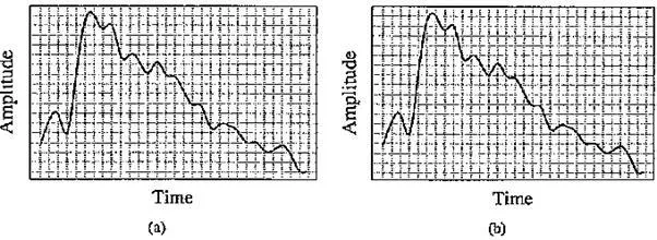
Since the graph in the above figure is two – dimensional, to fully digitize the signal shown we have to sample in each dimension — in time and in amplitude. Sampling means measuring the quantity we are interested in, usually at evenly spaced intervals. The first kind of sampling — using measurements only at evenly spaced time intervals — is simply called sampling (surprisingly), and the rate at which it is performed is called the sampling frequency. The following figure (a) shows this type of digitization.
Sampling and quantization: (a) sampling the analog signal in the time dimension; (b) quantization is sampling the analog signal in the amplitude dimension.
For audio, typical sampling rates are from 8 kHz (8,000 samples per second) to 48 kHz. The human ear can hear from about 20 Hz (a very deep rumble) to as much as 20 kHz; above this level, we enter the range of ultrasound. The human voice can reach approximately 4 kHz and we need to bound our sampling rate from below by at least double this frequency (see the discussion of the Nyquist sampling rate, below). Thus we arrive at the useful range about 8 to 40 or so kHz.
Sampling in the amplitude or voltage dimension is called quantization, shown in the above figure (b). While we have discussed only uniform sampling, with equally spaced sampling intervals, nonuniform sampling is possible. This is not used for sampling in time but is used for quantization (see the μ – law rule, below). Typical uniform quantization rates are 8 – bit and 16 – bit; 8 – bit quantization divides the vertical axis into 256 levels, and 16 – bit divides it into 65,536 levels.
To decide how to digitize audio data, we need to answer the following questions:
What is the sampling rate?
1. How finely is the data to be quantized, and is the quantization uniform?
2. How is audio data formatted (i.e., what is the file format)?
Nyquist Theorem
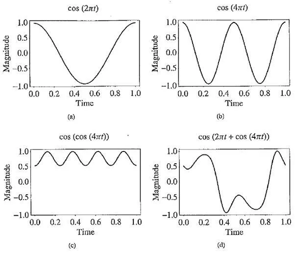
Signals can be decomposed into a sum of sinusoids, if we are willing to use enough sinusoids. The following figure shows how weighted sinusoids can build up quite a complex signal. Whereas frequency is an absolute measure, pitch is a perceptual, subjective quality of sound — generally, pitch is relative. Pitch and frequency are linked by setting the note A above middle C to exactly 440 Hz. An octave above that note corresponds to doubling the frequency and takes us to another A note. Thus, with the middle A on a piano (“A4” or “A440”) set to 440 Hz, the next A up is 880 Hz, one octave above.
Here, we define harmonics as any series of musical tones whose frequencies are integral multiples of the frequency of a fundamental tone. The following figure shows the appearance of these harmonics.
Now, if we allow noninteger multiples of the base frequency, we allow nori – A notes and have a complex resulting sound. Nevertheless, each sound is just made from sinusoids.
In computer graphics, much effort is aimed at masking such alias effects by various methods of antialiasing. An alias is any artifact that does not belong to the original signal. Thus, for correct sampling we must use a sampling rate equal to at least twice the maximum frequency content in the signal. This is called the Nyquist rate.
The Nyquist Theoremis named after Harry Nyquist, a famous mathematician who worked at Bell Labs. More generally, if a signal is band – limited — that is, if it has a lower limit f1
Building up a complex signal by superposing sinusoids
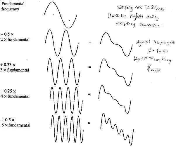
and an upper limit f1 of frequency components in the signal — then we need a sampling rate of at least 2(f2 – f1).
Suppose we have a fixed sampling rate. Since it would be impossible to recover frequencies higher than half the sampling rate in any event, most systems have an antialiasing filter that restricts the frequency content of the sampler’s input to a range at or below half the sampling frequency. Confusingly, the frequency equal to half the Nyquist rate is called the Nyquist frequency. Then for our fixed sampling rate, the Nyquist frequency is half the sampling rate. The highest possible signal frequency component has frequency equal to that of the sampling itself.
Note that the true frequency and its alias are located symmetrically on the frequency axis with respect to the Nyquist frequency pertaining to the sampling rate used. For this reason, the Nyquist frequency associated with the sampling frequency is often called the “folding” frequency. That is to say, if the sampling frequency is less than twice the true frequency, and is greater than the true frequency, then the alias frequency equals the sampling frequency
Aliasing: (a) a single frequency; (b) sampling at exactly the frequency produces a constant; (c) sampling at 1.5 times per cycle produced analiasfrequency that is perceived
minus the true frequency. For example, if the true frequency is 5.5 kHz and the sampling frequency is 8 kHz, then the alias frequency is 2.5 kHz:
As well, a frequency at double any frequency could also fit sample points. In fact, adding any positive or negative multiple of the sampling frequency to the true frequency always gives another, possible alias frequency, in that such an alias gives the same set of samples when sampled at the sampling frequency.
So, if again the sampling frequency is less than twice the true frequency and is less than the true frequency, then the alias frequency equals n times the sampling frequency minus the true frequency, where the n is the lowest integer that makes n times the sampling frequency larger than the true frequency. For example, when the true frequency is between 1.0 and 1.5 times the sampling frequency, the alias frequency equals the true frequency minus the sampling frequency.
Folding of sinusoid frequency sampled at 8,000 Hz. The folding frequency, shown dashed, is 4,000 Hz
In general, the apparent frequency of a sinusoid is the lowest frequency of a sinusoid that has exactly the same samples as the input sinusoid. The above figure shows the relationship of the apparent frequency to the input (true) frequency.
Signal – to – Noise Ratio (SNR)
Signal – to – noise ratio (often abbreviated SNR or S / N) is a measure used in science and engineering that compares the level of a desired signal to the level of background noise. It is defined as the ratio of signal power to the noise power. A ratio higher than 1:1 indicates more signal than noise. While SNR is commonly quoted for electrical signals, it can be applied to any form of signal (such as isotope levels in an ice core or biochemical signaling between cells).
The signal – to – noise ratio, the bandwidth, and the channel capacity of a communication channel are connected by the Shannon – Hartley theorem.
Signal – to – noise ratio is sometimes used informally to refer to the ratio of useful information to false or irrelevant data in a conversation or exchange. For example, in online discussion forums and other online communities, off – topic posts and spam are regarded as “noise” that interferes with the “signal” of appropriate discussion.
Signal – to – Quantization – Noise Ratio (SQNR)
Signal – to – Quantization – Noise Ratio (SQNR or SNqR) is widely used quality measure in analyzing digitizing schemes such as PCM (pulse code modulation) and multimedia codecs. The SQNR reflects the relationship between the maximum nominal signal strength and the quantization error (also known as quantization noise) introduced in the analog – to – digital conversion.
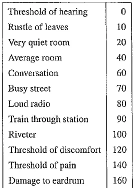
Table Magnitudes of common sounds, in decibels
Linear and Nonlinear Quantization
We mentioned above that samples are typically stored as uniformly quantized values. This is called linear format. However, with a limited number of bits available, it may be more sensible to try to take into account the properties of human perception and set up nonuniform quantization levels that pay more attention to the frequency range over which humans hear best.
Remember that here we are quantizing magnitude, or amplitude —- how loud the signal is. We already discussed an interesting feature of many human perception subsystems (as it were) — Weber’s Law — which states that the more there is, proportionately more must be added to discern a difference. Stated formally, Weber’s Law says that equally perceived differences have values proportional to absolute levels:
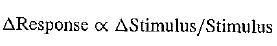
This means that, for example, if we can feel an increase in weight from 10 to 11 pounds, then if instead we start at 20 pounds, it would take 22 pounds for us to feel an increase in weight.
Inserting a constant of proportionality k, we have a differential equation that states

with response r and stimulus s. Integrating, we arrive at a solution
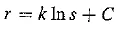
with constant of integration C. Stated differently, the solution is
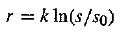
where so is the lowest level of stimulus that causes a response (r — 0 when s = so).
Thus, nonuniform quantization schemes that take advantage of this perceptual characteristic make use of logarithms. The idea is that in a log plot derived from the above equation, if we simply take uniform steps along the s axis, we are not mirroring the nonlinear response along the r axis.
Instead, we would like to take uniform steps along the r axis. Thus, nonlinear quantization works by first transforming an analog signal from the raw s space into the theoretical r space, then uniformly quantizing the resulting values. The result is that for steps near the low end of the signal, quantization steps are effectively more concentrated on the s axis, whereas for large values of s, one quantization step in r encompasses a wide range of s values.
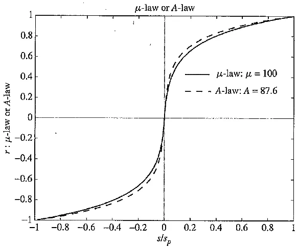
Such a law for audio is called μ – law encoding, or it – law, since it’s easier to write. A very similar rule, called A – law, is used in telephony in Europe.
The equations for these similar encodings are as follows:
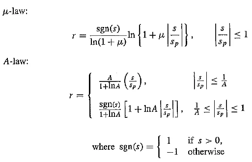
Nonlinear transform for audio signals
This technique is based on human perception — a simple form of “perceptual coder”. Interestingly, we have in effect also made use of the statistics of sounds we are likely to hear, which are generally in the low – volume range. In effect, we are asking for most bits to be assigned where most sounds occur — where the probability density is highest. So this type of coder is also one that is driven by statistics.
In summary, a logarithmic transform, called a “compressor” in the parlance of telephony, is applied to the analog signal before it is sampled and converted to digital (by an analog – to – digital, or AD, converter). The amount of compression increases as the amplitude of the input signal increases. The AD converter carries out a uniform quantization on the “compressed” signal. After transmission, since we need analog to hear sound, the signal is converted back, using a digital – to – analog (DA) converter, then passed through an “expander” circuit that reverses the logarithm. The overall transformation is called companding. Now a days, companding can also be carried out in the digital domain.
The µ – law in audio is used to develop a nonuniform quantization rule for sound. In general, we would like to put the available bits where the most perceptual acuity (sensitivity to small changes) is. Ideally, bit allocation occurs by examining a curve of stimulus versus response for humans. Then we try to allocate bit levels to intervals for which a small change in stimulus produces a large change in response.
That is, the idea of companding reflects a less specific idea used in assigning bits to signals: put the bits where they are most needed to deliver finer resolution where the result can be perceived. This idea militates against simply using uniform quantization schemes, instead favoring nonuniform schemes for quantization. The µ – law (or A – law) for audio is an application of this idea.
Audio Filtering
An audio filter is a frequency dependent amplifier circuit, working in the audio frequency range, 0 Hz to beyond 20 kHz. Many types of filters exist for applications including graphic equalizers, synthesizers, sound effects, CD players and virtual reality systems.
Being a frequency dependent amplifier, in its most basic form, an audio filter is designed to amplify, pass or attenuate (negative amplification) some frequency ranges. Common types include low – pass, which pass through frequencies below their cutoff frequencies, and progressively attenuates frequencies above the cutoff frequency. A high – pass filter does the opposite, passing high frequencies above the cutoff frequency, and progressively attenuating frequencies below the cutoff frequency. A bandpass filter passes frequencies between its two cutoff frequencies, while attenuating those outside the range. A band – reject filter attenuates frequencies between its two cutoff frequencies, while passing those outside the ‘reject’ range.
An all – pass filter, passes all frequencies, but affects the phase of any given sinusoidal component according to its frequency. In some applications, such as in the design of graphic equalizers or CD players, the filters are designed according to a set of objective criteria such as pass band, pass band attenuation, stop band, and stop band attenuation, where the pass bands are the frequency ranges for which audio is attenuated less than a specified maximum, and the stop bands are the frequency ranges for which the audio must be attenuated by a specified minimum.
In more complex cases, an audio filter can provide a feedback loop, which introduces resonance (ringing) alongside attenuation. Audio filters can also be designed to provide gain (boost) as well as attenuation.
In other applications, such as with synthesizers or sound effects, the aesthetic of the filter must be evaluated subjectively.
Audio filters can be implemented in analog circuitry as analog filters or in DSP code or computer software as digital filters. Generically, the term ‘audio filter’ can be applied to mean anything which changes the timbre, or harmonic content of an audio signal.
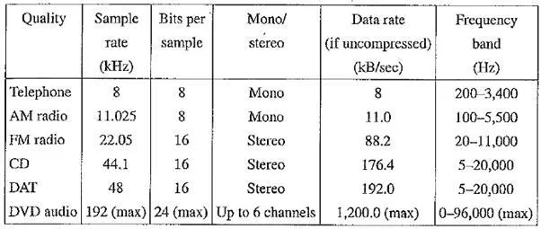
Audio Quality versus Data Rate
The uncompressed data rate increases as more bits are used for quantization. Stereo information, as opposed to mono, doubles the amount of bandwidth (in bits per second) needed to transmit a digital audio signal. The following table shows how audio quality is related to data rate and bandwidth.
The term bandwidth, in analog devices, refers to the part of the response or transfer function of a device that is approximately constant, or flat, with the x – axis being the frequency and the y – axis equal to the transfer function. Half – power bandwidth (HPBW) refers to the bandwidth between points when the power falls to half the maximum power. Since 10 logI0(0.5) ≈ – 3.0, the term -3 dB bandwidth is also used to refer to the HPBW.
So for analog devices, the bandwidth is expressed in frequency units, called Hertz (Hz), which is cycles per second. For digital devices, on the other hand, the amount of data that can be transmitted in a fixed bandwidth is usually expressed in bits per second (bps) or bytes per amount of time. For either analog or digital, the term expresses the amount of data that can be transmitted in a fixed amount of time.
Table Data rate and bandwidth in sample audio applications
Telephony uses μ – law (or u – law) encoding, or A – law in Europe. The other formats use linear quantization. Using the μ – law rule, the dynamic range of digital telephone signals is effectively improved from 8 bits to 12 or 13.
Sometimes it is useful to remember the kinds of data rates in the above table in terms of bytes per minute. For example, the uncompressed digital audio signal for CD – quality stereo sound is 10.6 megabytes per minute — roughly 10 megabytes — per minute.
Synthetic Sounds
Synthetic sounds are produced by electronic hardware or digital hardware simulations of oscillators and filters. Sound is created entirely from nothing using equations which express some functions of time and there need not be any other data. Synthesizers produce audio waveforms with dynamic shape, spectrum and amplitude characteristics. They may be generated for sounds corresponding to real instruments like brass or piano, or for completely imaginary ones. The combination of sequencers and synthesizers is mainly responsible for the genre of techno and dance music but can produce ambient backgrounds too. Synthesizers also play a non – musical role for creating sound effects like rain, wind, thunder or just about anything you care to imagine. The power of synthetic sound is that it is unlimited in potential, just as long as you know how to figure out the equations needed for a certain sound.
Frequency modulation: (a) a single frequency; (b) twice the frequency; (c) usually, FM is carried out using a sinusoid argument to a sinusoid; (d) a more complex form arises from a carrier frequency 2nt and a modulating frequency 4irt cosine inside the sinusoid
For example, it is useful to be able to change the key -— suppose a song is a bit too high for your voice. A wave table can be mathematically shifted so that it produces lower – pitched sounds. However, this kind of extrapolation can be used only just so far without sounding wrong. Wave tables often include sampling at various notes of the instrument, so that a key change need not be stretched too far. Wave table synthesis is more expensive than FM synthesis, partly because the data storage needed is much larger.

Comments are closed