To be transmitted, sampled audio information must be digitized, and here we look at some of the details of this process. Once the information has been quantized, it can then be transmitted or stored. We go through a few examples in complete detail, which helps in understanding what is being discussed.

Coding of Audio

Quantization and transformation of data are collectively known as coding of the data. For audio, the μ – law technique for companding audio signals is usually combined with a simple algorithm that exploits the temporal redundancy present in audio signals. Differences in signals between the present and a previous time can effectively reduce the size of signal values and, most important, concentrate the histogram of pixel values (differences, now) into a much smaller range. The result of reducing the variance of values is that lossless compression methods that produce a bitstream with shorter bit lengths for more likely values, fare much better and produce a greatly compressed bitstream.

In general, producing quantized sampled output for audio is called Pulse Code Modulation, or PCM. The differences version is called DPCM (and a crude but efficient variant is called DM). The adaptive version is called ADPCM, and variants that take into account speech properties follow from these.

Pulse Code Modulation

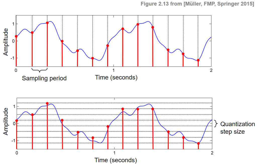
PCM in General. Audio is analog — the waves we hear travel through the air to reach our ear drums. We know that the basic techniques for creating digital signals from analog ones consist of sampling and quantization. Sampling is invariably done uniformly — we select a sampling rate and produce one value for each sampling time.

In the magnitude direction, we digitize by quantization, selecting breakpoints in magnitude and remapping any value within an interval to one representative output level. The set of interval boundaries is sometimes called decision boundaries, and the representative values are called reconstruction levels.

We say that the boundaries for quantizer input intervals that will all be mapped into the same output level form a coder mapping, and the representative values that are the output values from a quantizer are a decoder mapping. Since we quantize, we may choose to create either an accurate or less accurate representation of sound magnitude values. Finally, we may wish to compress the data, by assigning a bitstream that uses fewer bits for the most prevalent signal values.

Every compression scheme has three stages:

Transformation. The input data is transformed to a new representation that is easier or more efficient to compress. For example, in Predictive Coding, (discussed later in the chapter) we predict the next signal from previous ones and transmit the prediction error.

Loss. We may introduce loss of information. Quantization is the main lossy step. Here we use a limited number of reconstruction levels, fewer than in the original signal. Therefore, quantization necessitates some loss of information.

·         Coding. Here, we assign a codeword (thus forming a binary bitstream) to each output level or symbol. This could be a fixed – length code or a variable – length code, such as Huffman coding.

For audio signals, we first consider PCM, the digitization method. That enables us to consider Lossless Predictive Coding as well as the DPCM scheme; these “methods use differential coding. We also look at the adaptive, version, ADPCM, which is meant to provide better compression.

Pulse Code Modulation, is a formal term for the sampling and quantization we have already been using. Pulse comes from an engineer’s point of view that the resulting digital signals can be thought of as infinitely narrow vertical “pulses”. As an example of PCM, audio samples on a CD might be sampled at a rate of 44.1 kHz, with 16 bits per sample.

PCM in Speech Compression. The so – called compressor and expander stages for speech signal processing, for telephony. For this application, signals are first transformed using the μ – law (or A – law for Europe) rule into what is essentially a logarithmic scale. Only then is PCM, using uniform quantization, applied. The result is that finer increments in sound volume are used at the low – volume end of speech rather than at the high – volume end, where we can’t discern small changes in any event.

Assuming a bandwidth for speech from about 50 Hz to about 10 kHz, the Nyquist rate . would dictate a sampling rate of 20 kHz. Using uniform quantization without companding, the minimum sample size we could get away with would likely be about 12 bits. Hence, for mono speech transmission the bitrate would be 240 kbps. With companding, we can safely reduce the sample size to 8 bits with the same perceived level of quality and thus reduce the bitrate to 160 kbps. However, the standard approach to telephony assumes that the highest – frequency audio signal we want to reproduce is about 4 kHz. Therefore, the sampling rate is only 8 kHz, and the companded bitrate thus reduces to only 64 kbps.

We must also address two small wrinkles to get this comparatively simple form of speech compression right. First because only sounds up to 4 kHz are to be considered, all other frequency content must be noise. Therefore, we should remove this high – frequency content from the analog input signal. This is done using a band – limiting filter that blocks out high frequencies as well as very low ones. The “band” of not – removed (“passed”) frequencies are what we wish to keep. This type of filter is therefore also called a band – pass filter.

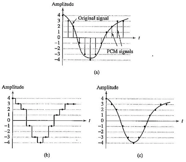
Second, once we arrive at a pulse signal, such as the one in the following figure, we must still perform digital – to – analog conversion and then construct an output analog signal. But

Pulse code modulation (PCM): (a) original analog signal and its corresponding PCM signals; (b) decoded staircase signal; (c) reconstructed signal after low – pass filtering

PCM signal encoding and decoding

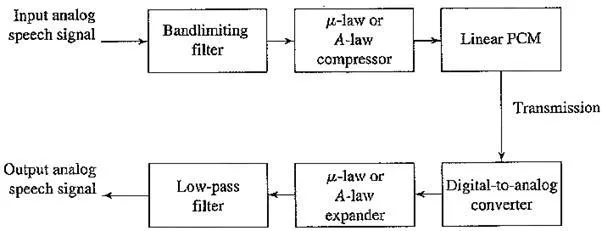
The signal we arrive at is effectively the staircase. This type of discontinuous signal contains not just frequency components due to the original signal but, because of the sharp corners, also a theoretically infinite set of higher – frequency components (from the theory of Fourier analysis, in signal processing). We know these higher frequencies are extraneous. Therefore, the output of the digital – to – analog converter is in turn passed to a low – pass filter, which allows only frequencies up to the original maximum to be retained. The above figure shows the complete scheme for encoding and decoding telephony signals as a schematic.

A – law or μ – law PCM coding is used in the older International Telegraph and Telephone Consultative Committee (CCITT) standard G.711, for digital telephony. This CCITT standard is now subsumed into standards promulgated by a newer organization, the International Telecommunication Union (ITU).

Differential Coding of Audio

Audio is often stored not in simple PCM but in a form that exploits differences. For a start, differences will generally be smaller numbers and hence offer the possibility of using fewer bits to store.

An advantage of forming differences is that the histogram of a difference signal is usually considerably more peaked than the histogram for the original signal. For example, as an extreme case, the histogram for a linear ramp signal that has constant slope is uniform, whereas the histogram for the derivative of the signal (I.e., the differences, from sampling point to sampling point) consists of a spike at the slope value.

Generally, if a time – dependent signal has some consistency over time (temporal redundancy), the difference signal — subtracting the current sample from the previous one — will have a more peaked histogram, with a maximum around zero. Consequently, if we then go on to assign bitstring codewords to differences, we can assign short codes to prevalent values and long codewords to rarely occurring ones.

To begin with, consider a lossless version of this scheme. Loss arises when we quantize. If we apply no quantization, we can still have compression — via the decrease in the variance of values that occurs in differences, compared to the original signal. With quantization, Predictive Coding becomes DPCM, a lossy method; we’ll also try out that scheme.

Lossless Predictive Coding

Predictive coding simply means transmitting differences — we predict the next sample as being equal to the current sample and send not the sample itself but the error involved in making this assumption. That is, if we predict that the next sample equals the previous one, then the error is just the difference between previous and next. Our prediction scheme could also be more complex.

However, we do note one problem. Suppose our integer sample values are in the range 0..255. Then differences could be as much as —255 ..255. So we have unfortunately increased our dynamic range (ratio of maximum to minimum) by a factor of two: we may well need more bits than we needed before to transmit some differences. Fortunately, we can use a trick to get around this problem, as we shall see.

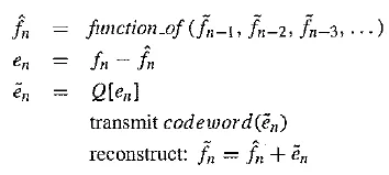
So, basically, predictive coding consists of finding differences and transmitting them, using a PCM system. First, note that differences of integers will at least be integers. Let’s formalize our statement of what we are doing by defining the integer signal as the set of values fn. Then we predict values fn as simply the previous value, and we define the error en as the difference between the actual and predicted signals:

We certainly would like our error value ento be as small as possible. Therefore, we would wish our prediction to be as close as possible to the actual signal fn But for a particular sequence of signal values, some function of a few of the previous values, f n-1, f n-2, f n-3 etc., may provide a better prediction of fn. Typically, a linear predictor function is used:

Such a predictor can be followed by a truncating or rounding operation to result in integer values. In fact, since now we have such coefficients a n – k available, we can even change them adaptively.

The idea of forming differences is to make the histogram of sample values more peaked. For example, the following figure (a) plots 1 second of sampled speech at 8 kHz, with magnitude resolution of 8 bits per sample.

A histogram of these values is centered on zero, as in the following figures (b) and (c) shows the histogram for corresponding speech signal differences: difference values are much more clustered around zero than are sample values themselves. As a result, a method that

Differencing concentrates the histogram: (a) digital speech signal; (b) histogram of digital speech signal values; (c) histogram of digital speech signal differences

assigns short code words to frequently occurring symbols will assign a short code to zero and do rather well. Such a coding scheme will much more efficiently code sample differences than samples themselves, and a similar statement applies if we use a more sophisticated predictor than simply the previous signal value.

However, we are still left with the problem of what to do if, for some reason, a particular set of difference values does indeed consist of some exceptional large differences. A clever solution to this difficulty involves defining two new codes to add to our list of difference values, denoted SU and SD, standing for Shift – Up and Shift – Down. Some special values will be reserved for them.

Suppose samples are in the range 0..255, and differences are in —255.. 255. Define SU and SD as shifts by 32. Then we could in fact produce codewords for a limited set of signal differences, say only the range —15.. 16. Differences (that inherently are in the range —255 .. 255) lying in the limited range can be coded as is, but if we add the extra two values for SU, SD, a value outside the range —15 .. 16 can be transmitted as a series of shifts, followed by a value that is indeed inside the range —15..16. For example, 100 is transmitted as SU, – SU, SU, 4, where (the codes for) SU and for 4 are what are sent.

Lossless Predictive Coding is… lossless! That is, the decoder produces the same signals as the original. It is helpful to consider an explicit scheme for such coding considerations, so let’s do that here (we won’t use the most complicated scheme, but we’ll try to carry out an entire calculation). As a simple example, suppose we devise a predictor for fnas follows:

Then the error en (or a codeword for it) is what is actually transmitted.

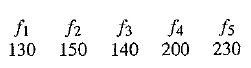
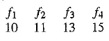
Let’s consider an explicit example. Suppose we wish to code the sequence f1, f2, f3, f4, f5 = 21, 22, 27, 25, 22. For the purposes of the predictor, we’ll invent an extra signal value f0, equal to f1 = 21, and first transmit this initial value, uncoded; after all, every coding scheme has the extra expense of some header information. Then the first error, e1, is zero, and subsequently

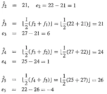
The error does center on zero, we see, and coding (assigning bitstring codewords) will be efficient.

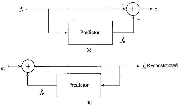
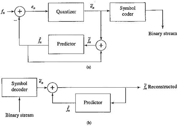
Schematic diagram for Predictive Coding: (a) encoder; (b) decoder

Therefore, the predictor must involve a memory. At the least, the predictor includes a circuit for incorporating a delay in the signal, to store fn – 1.

DPCM

Differential Pulse Code Modulation is exactly the same as Predictive Coding, except that it incorporates a quantizer step. Quantization is as in PCM and can be uniform or nonuniform. One scheme for analytically determining the best set of nonuniform quantizer steps is the Lloyd – Max quantizer, named for Stuart Lloyd and Joel Max, which is based on a least – squares minimization of the error term.

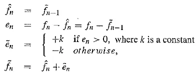
Here we should adopt some nomenclature for signal values. We shall call the original signal fn, the predicted signal fn, and the quantized, reconstructed signal fn. How DPCM operates is to form the prediction, form an error en by subtracting the prediction from the actual signal, then quantize the error to a quantized version, en. The equations that describe DPCM are as follows:

Codewords for quantized error values en are produced using entropy coding, such as Huffman coding.

Notice that the predictor is always based on the reconstructed, quantized version of the signal: the reason for this is that the encoder side is not using any information not available to the decoder side. Generally, if by mistake we made use of the actual signals fn in the predictor instead of the reconstructed ones fn, quantization error would tend to accumulate and could get worse rather than being centered on zero.

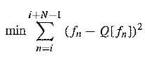
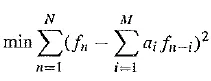
The main effect of the coder – decoder process is to produce reconstructed, quantized signal values.The “distortion” is the average squared errorand one often sees diagrams of distortion versus the number of bit levels used. A Lloyd – Max quantizer will do better (have less distortion) than a uniform quantizer. For any signal, we want to choose the size of quantization steps so that they correspond to the range (the maximum and minimum) of the signal. Even using a uniform, equal – step quantization will naturally do better if we follow such a practice. For speech, we could modify quantization steps as we go, by estimating the mean and variance of a patch of signal values and shifting quantization steps accordingly, for every block of signal values. That is, starting at time i we could take a block of N values fn and try to minimize the quantization error:

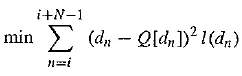
Since signal differences are very peaked, we could model them using a Laplacian probability distribution function, which is also strongly peaked at zero: it looks likefor variance a . So typically, we assign quantization steps for a quantizer with nonuniform steps by assuming that signal differences, dn, say, are drawn from such a distribution and then choosing steps to minimize

This is a least – squares problem and can be solved iteratively using the Lloyd – Max quantizer.

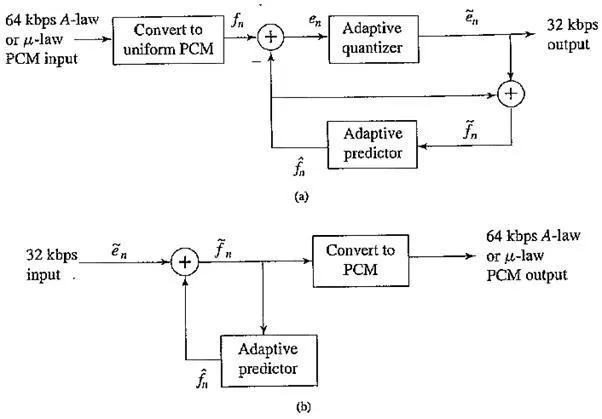
The following figure shows a schematic diagram for the DPCM coder and decoder. As is common in such diagrams, several interesting features are more or less not indicated. First, we notice that the predictor makes use of the reconstructed, quantized signal values fn, not actual signal values fn — that is, the encoder simulates the decoder in the predictor path. The quantizer can be uniform or non – uniform.

The box labeled “Symbol coder” in the block diagram simply means a Huffman coder. The prediction value fn is based on however much history the prediction scheme requires: we need to buffer previous values of f to form the prediction. Notice that the quantization noiseis equal to the quantization effect on the error term, en – en

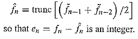
It helps us explicitly understand the process of coding to look at actual numbers. Suppose we adopt a particular predictor as follows:

Schematic diagram for DPCM: (a) encoder; (b) decoder

Let us use the particular quantization scheme

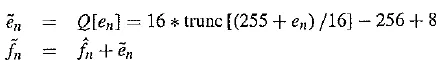
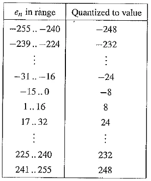
First, we note that the error is in the range —255 ..255 — that is, 511 levels are possible for the error term. The quantizer takes the simple course of dividing the error range into 32 patches of about 16 levels each. It also makes the representative reconstructed value for each patch equal to the midway point for each group of 16 levels.

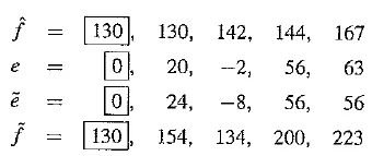
The following table gives output values for any of the input codes: 4 – bit codes are mapped to 32 reconstruction levels in a staircase fashion. (Notice that the final range includes only 15 levels, not 16.) As an example stream of signal values, consider the set of values

We prepend extra values f = 130 in the datastream that replicate the first value, f1, and initialize with quantized error e1 = 0, so that we ensure the first reconstructed value is

DPCM quantizer reconstruction levels

DM

DM stands for Delta Modulation, a much – simplified version of DPCM often used as a quick analog – to – digital converter. We include this scheme here for completeness.

Uniform – Delta DM. The idea in DM is to use only a single quantized error value, either positive or negative. Such a 1 – bit coder thus produces coded output that follows the original signal in a staircase fashion. The relevant set of equations is as follows:

Note that the prediction simply involves a delay.

Again, let’s consider actual numbers. Suppose Suppose signal values are as follows:

We also define an exact reconstructed value f1=10.

Suppose we use a step value k = 4. Then we arrive at the following values:

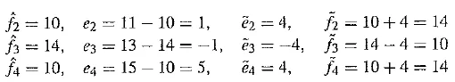
We see that the reconstructed set of values 10, 14, 10, 14 never strays far from the correct set 10, 11, 13, 15.

Nevertheless, it is not difficult to discover that DM copes well with more or less constant signals, but not as well with rapidly changing signals. One approach to mitigating this problem is to simply increase the sampling, perhaps to many times the Nyquist rate. This scheme can work well and makes DM a very simple yet effective analog – to – digital converter.

Adaptive DM. However, if the slope of the actual signal curve is high, the staircase approximation cannot keep up. A straightforward approach to dealing with a steep curve is to simply change the step size k adoptively — that is, in response to the signal’s current properties.

ADPCM

Adaptive DPCM takes the idea of adapting the coder to suit the input much further. Basically, two pieces make up a DPCM coder: the quantizer and the predictor. Above, in Adaptive DM, we adapted the quantizer step size to suit the input. In DPCM, we can adoptively modify the quantizer, by changing the step size as well as decision boundaries in a nonuniform quantizer.

We can carry this out in two ways: using the properties of the input signal (called forward adaptive quantization), or the properties of the quantized output. For if quantized errors become too large, we should change the nonuniform Lloyd – Max quantizer (this is called backward adaptive quantization).

We can also adapt the predictor, again using forward or backward adaptation. Generally, making the predictor coefficients adaptive is called Adaptive Predictive Coding (APC). It is interesting to see how this is done. Recall that the predictor is usually taken to be a linear function of previously reconstructed quantized values, fn. The number of previous values used is called the order of the predictor.

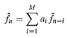
However we can get into a difficult situation if we try to change the prediction coefficients that multiply previous quantized values, because that makes a complicated set of equations to solve for these coefficients. Suppose we decide to use a least – squares approach to solving a minimization, trying to find the hest values of the ai:

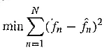
where here we would sum over a large number of samples fn for the current patch of speech, say. But because fn depends on the quantization, we have a difficult problem to solve. Also, we should really be changing the fineness of the quantization at the same time, to suit the signal’s changing nature; this makes things problematical.

Instead, we usually resort to solving the simpler problem that results from using not fn in the prediction hut simply the signal fn itself. This is indeed simply solved, since, explicitly writing in terms of the coefficients a1, we wish to solve

Differentiation with respect to each of the a, and setting to zero produces a linear system of M equations that is easy to solve. (The set of equations is called the Wiener – Hopf equations.) Thus we indeed find a simple way to adaptively change the predictor as we go. For speech signals, it is common to consider blocks of signal values, just as for image coding, and adaptively change the predictor, quantizer, or both. If we sample at 8 kHz, a common block size is 128 samples — 16 msec of speech.

Schematic diagram for: (a) ADPCM encoder; (b) decoder