The emergence of multimedia technologies has made digital libraries a reality. Nowadays, libraries, museums, film studios, and governments are converting more and more data and archives into digital form. Some of the data (e.g., precious books and paintings) indeed need to be stored without any loss.
As a start, suppose we want to encode the call numbers of the 120 million or so items in the Library of Congress (a mere 20 million, if we consider just books). Why don’t we just transmit each item as a 27 – bit number, giving each item a unique binary code (since 227 > 120,000,000)?
The main problem is that this “great idea” requires too many bits. And in fact there exist many coding techniques that will effectively reduce the total number of bits needed to represent the above information. The process involved is generally referred to as compression.
In Chapter, we had a beginning look at compression schemes aimed at audio. There, we had to first consider the complexity of transforming analog signals to digital ones, whereas here, we shall consider that we at least start with digital signals. For example, even though we know an image is captured using analog signals, the file produced by a digital camera is indeed digital. The more general problem of coding (compressing) a set of any symbols, not just byte values, say, has been studied for a long time.
Getting back to our Library of Congress problem, it is well known that certain parts of call numbers appear more frequently than others, so it would be more economic to assign fewer bits as their codes. This is known as variable – length coding (VLC) — the more frequently – appearing symbols are coded with fewer bits per symbol, and vice versa. As a result, fewer bits are usually needed to represent the whole collection.
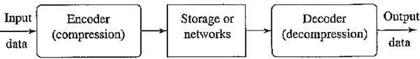
In this chapter we study the basics of information theory and several popular lossless compression techniques. The following figure depicts a general data compression scheme, in which compression is performed by an encoder and decompression is performed by a decoder.
We call the output of the encoder codes or codewords. The intermediate medium could either be data storage or a communication / computer network. If the compression and decompression processes induce no information loss, the compression scheme is lossless; otherwise, it is lossy. The next several chapters deal with lossy compression algorithms as they are commonly used for image, video, and audio compression. Here, we concentrate on lossless compression.
A general data compression scheme
If the total number of bits required to represent the data before compression is B0 and the total number of bits required to represent the data after compression is B1, then we define the compression ratio as
Compression ratio = B0 / B1
In general, we would desire any codec (encoder / decoder scheme) to have a compression ratio much larger than 1.0. The higher the compression ratio, the better the lossless compression scheme, as long as it is computationally feasible.
Histograms for two gray – level images
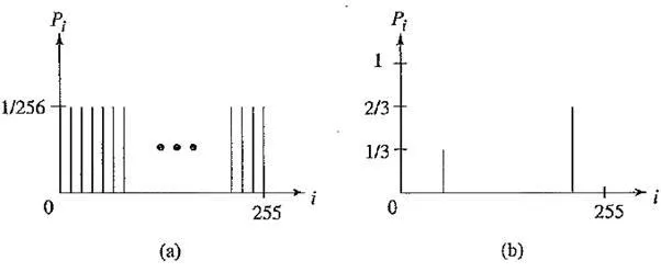
The above figure (a) shows the histogram of an image with uniform distribution of gray – level intensities, — that is, Pi = 1 / 256. Hence, the entropy of this image is
As can be seen, the entropy Equation is a weighted sum of terms Log2 i / Pi; hence it represents the average amount of information contained per symbol in the source S. For a memoryless source2 S, the entropy n represents the minimum average number of bits required to represent each symbol in S. In other words, it specifies the lower bound for the average number of bits to code each symbol in S.
If we use l to denote the average length (measured in bits) of the code words produced by the encoder, the Shannon Coding Theorem states that the entropy is the best we can do (under certain conditions):
Coding schemes aim to get as close as possible to this theoretical lower bound,
It is interesting to observe that in the above uniform – distribution example we found that η = 8 –minimum average number of bits to represent each gray – level intensity is at least 8. No compression is possible for this image! In the context of imaging, this will correspond to the “worst case,” where neighboring pixel values have no similarity.
The above figure (b) shows the histogram of another image, in which 1 / 3 of the pixels are rather dark and 2 / 3 of them are rather bright. The entropy of this image is
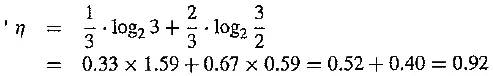
In general, the entropy is greater when the probability distribution is flat and smaller when it is more peaked.