Since the entropy indicates the information content in an information source 5, it leads to a family of coding methods commonly known as entropy coding methods. As described earlier, variable – length coding (VLC) is one of the best – known such methods. Here, we will study the Shannon – Fano algorithm, Huffman coding, and adaptive Huffman coding.

Shannon – Fano Algorithm

The Shannon – Fano algorithm was independently developed by Shannon at Bell Labs and Robert Fano at MIT. To illustrate the algorithm, let’s suppose the symbols to be coded are the characters in the word HELLO. The frequency count of the symbols is

The encoding steps of the Shannon – Fano algorithm can be presented in the following top – down manner;

·         Sort the symbols according to the frequency count of their occurrences.

·         Recursively divide the symbols into two parts, each with approximately the same number of counts, until all parts contain only one symbol.

A natural way of implementing the above procedure is to build a binary tree.As a convention, let’s assign bit 0 to its left branches and 1 to the right branches.

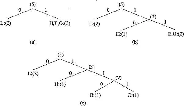
Coding tree for HELLO by the Shannon – Fano algorithm

Initially, the symbols are sorted as LHEO. As the above figure shows, the first division yields two parts: (a) L with a count of 2, denoted as L:(2); and (b) H, E and O with a total count of 3, denoted as H,E,0:(3). The second division yields H:(l) and E,0:(2). The last division is E:(l) and O:(l).

Table summarizes the result, showing each symbol, its frequency count, information content {log 2 ~ 1, resulting codeword, and the number of bits needed to encode each symbol in the word HELLO. The total number of bits used is shown at the bottom. To revisit the previous discussion on entropy, in this case,

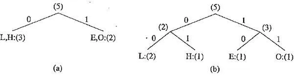
Table One result of performing the Shannon – Fano algorithm on HELLO

Another coding tree for HELLO by the Shannon – Fano algorithm

This suggests that the minimum average number of bits to code each character in the word HELLO would be at least 1.92. In this example, the Shannon – Fano algorithm uses an average of 10 / 5 = 2 bits to code each symbol, which is fairly close to the lower bound of 1.92. Apparently, the result is satisfactory.

It should be pointed out that the outcome of the Shannon – Fano algorithm is not necessarily unique. For instance, at the first division in the above example, it would be equally valid to divide into the two parts L, H:(3) and E,0:(2). This would result in the coding in the above figure. The following table shows the codewords are different now. Also, these two sets of code  words may behave differently when errors are present. Coincidentally, the total number of bits required to encode the world HELLO remains at 10.

The Shannon – Fano algorithm delivers satisfactory coding results for data compression, but it was soon outperformed and overtaken by the Huffman coding method.

Huffman Coding

First presented by David A. Huffman in a 1952 paper, this method attracted an over whelming amount of research and has been adopted in many important and / or commercial applications, such as fax machines, JPEG, and MPEG.

In contradistinction to Shannon – Fano, which is top – down, the encoding steps of the Huffman algorithm are described in the following bottom – up manner. Let’s use the same example word, HELLO. A similar binary coding tree will be used as above, in which the left branches are coded 0 and right branches 1. A simple list data structure is also used.

Table Another result of performing the Shannon – Fano algorithm on HELLO

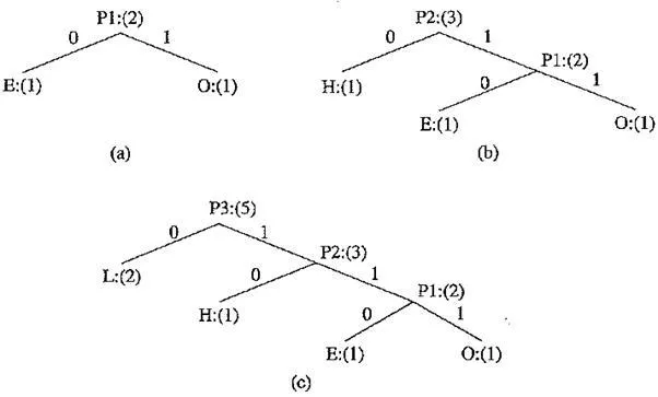
Coding tree for HELLO using the Huffman algorithm

ALGORITHM HUFFMAN CODING

·         Initialization: put all symbols on the list sorted according to their frequency counts.

·         Repeat until the list has only one symbol left.

·         From the list, pick two symbols with the lowest frequency counts. Form a Huffman subtree that has these two symbols as child nodes and create a parent node for them.

·         Assign the sum of the children’s frequency counts to the parent and insert it into the list, such that the order is maintained.

·         Delete the children from the list.

Assign a codeword for each leaf based on the path from the root.

In the above figure, new symbols PI, P2, P3 are created to refer to the parent nodes in the Huffman coding tree. The contents in the list are illustrated below:

After initialization:L H E O

After iteration (a):L PI H

After iteration (b):L P2

After iteration (c):P3

For this simple example, the Huffman algorithm apparently generated the same coding ‘result as one of the Shannon – Fano results shown in the following figure, although the results are usually better. The average number of bits used to code each character is also 2, (i.e., (1 + 1+2 + 3 + 3) / 5 = 2). As another simple example, consider a text string containing a set of characters and their frequency counts as follows: A : (15), B : (7), C : (6), D : (6) and E : (5). It is easy to show that the Shannon – Fano algorithm needs a total of 89 bits to encode this string, whereas the Huffman algorithm needs only 87.’ .1

As shown above, if correct probabilities (“prior statistics”) are available and accurate, the Huffman coding method produces good compression results. Decoding for the Huffman coding is trivial as long as the statistics and / or coding tree are sent before the data to be compressed (in the file header, say). This overhead becomes negligible if the data file is sufficiently large.

The following are important properties of Huffman coding:

·         Unique prefix property.No Huffman code is a prefix of any other Huffman code.
For instance, the code 0 assigned to L is not a prefix of the code 10 for H or 110 for E or 111 for O; nor is the code 10 for H a prefix of the code 110 forE or 111 for O. It turns out that the unique prefix property is guaranteed by the above

Huffman algorithm, since it always places all input symbols at the leaf nodes of theHuffman tree. The Huffman code is one of the prefix codes for which the unique prefix property holds. The code generated by the Shannon – Fano algorithm is another such example.

This property is essential and also makes for an efficient decoder, since it precludes any ambiguity in decoding. In the above example, if a bit 0 is received, the decoder can immediately produce a symbol L without waiting for any more bits to be transmitted.

·         Optimality.The Huffman code is a minimum – redundancy code, as shown in Huffman’s 1952 paper. It has been proven that the Huffman code is optimal for a given data model (i.e., a given, accurate, probability distribution):

1.      The two least frequent symbols will have the same length for their Huffman codes, differing only at the last bit. This should be obvious from the above algorithm.

2.      Symbols that occur more frequently will have shorter Huffman codes than symbols that occur less frequently. Namely, for symbols Si and sj, if pi ≥ pj then li ≥ lj, where li is the number of bits in the codeword for si.

3.      It has been shown that the average code length for an information source S is strictly less than η + 1. Combined with the above Eq. we have

Extended Huffman Coding.The discussion of Huffman coding so far assigns each symbol a codeword that has an integer bit length. As stated earlier, log2 1 / pt indicates the amount of information contained in the information source Sj, which corresponds to the number of bits needed to represent it. When a particular symbol si has a large probability (close to 1.0), log2 1 / pt will be close to 0, and assigning one bit to represent that symbol will be costly. Only when the probabilities of all symbols can be expressed as 2 – k, where & is a positive integer, would the average length of codewords be truly optimal -— that is, 1 = 7). Clearly, l > n in most cases, One way to address the problem of integral codeword length is to group several symbols and assign a single codeword to the group. Huffman coding of this type is called Extended Huffman Coding [2]. Assume an information source has alphabet S = {s1, s2,… , s„}. If k symbols are grouped together, then the extended alphabet is

Note that the size of the new alphabet S(k) is nk. If k is relatively large (e.g., k > 3), then for most practical applications where n >> 1, nk would be a very large number, implying a huge symbol table. This overhead makes Extended Huffman Coding impractical.

If the entropy of S is η, then the average number of bits needed for each symbol in S is now

so we have shaved quite a bit from the coding schemes’ bracketing of the theoretical best limit. Nevertheless, this is not as much of an improvement over the original Huffman coding (where group size is 1) as one might have hoped for.

Adaptive Huffman Coding

The Huffman algorithm requires prior statistical knowledge about the information source, and such information is often not available. This is particularly true in multimedia applications, where future data is unknown before its arrival, as for example in live (or streaming) audio and video. Even when the statistics are available, the transmission of the symbol table could represent heavy overhead.

For the non – extended version of Huffman coding, the above discussion assumes a so – called order – 0 model — that is, symbols / characters were treated singly, without any context or history maintained. One possible way to include contextual information is to examine k preceding (or succeeding) symbols each time; this is known as an order – k model. For example, an order – 1 model can incorporate such statistics as the probability of “qu” in addition to the individual probabilities of “q” and “u”. Nevertheless, this again implies that much more statistical data has to be stored and sent for the order – & model when k > 1.

The solution is to use adaptive compression algorithms, in which statistics are gathered and updated dynamically as the datastream arrives. The probabilities are no longer based on prior knowledge but on the actual data received so far. The new coding methods are “adaptive” because, as the probability distribution of the received symbols changes, symbols will be given new (longer or shorter) codes. This is especially desirable for multimedia data, when the content (the music or the color of the scene) and hence the statistics can change rapidly.

As an example, we introduce the Adaptive Huffman Coding algorithm in this section. Many ideas, however, are also applicable to other adaptive compression algorithms.

PROCEDURE

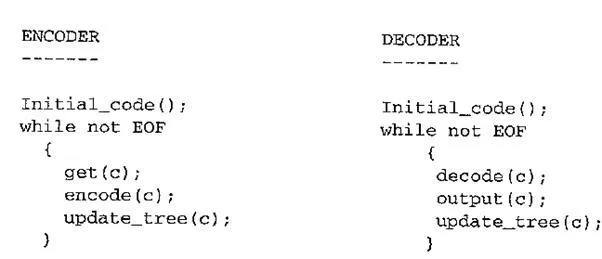
Procedures for Adaptive Huffman Coding

·         Initial _ code assigns symbols with some initially agreed – upon codes, without any prior knowledge of the frequency counts for them. For example, some conventional code such as ASCII may be used for coding character symbols.

·         update _ tr ee is a procedure for constructing an adaptive Huffman tree. It basically does two things: it increments the frequency counts for the symbols (including any new ones), and updates the configuration of the tree.

·         The Huffman tree must always maintain its sibling property — that is, all nodes (internal and leaf) are arranged in the order of increasing counts. Nodes are numbered in order from left to right, bottom to top. If the sibling property is about to be violated, a swap procedure is invoked to update the tree by rearranging the nodes.

·         When a swap is necessary, the farthest node with count N is swapped with the node whose count has just been increased to TV + 1. Note that if the node with count N is not a leaf – node — it is the root of a subtree — the entire subtree will go with it during the swap.

The encoder and decoder must use exactly the same Initial code and update routines.

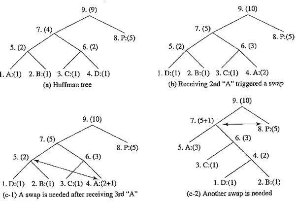
The following figure depicts a Huffman tree with some symbols already received. Another figure shows the updated tree after an additional A (i.e., the second A) was received. This increased the count of As to N + 1 — 2 and triggered a swap. In this case, the farthest node with count N = 1 was D:(l). Hence, A:(2) and D:(l) were swapped.

Apparently, the same result could also be obtained by first swapping A:(2) with B:(l), then with C:(l), and finally with D:(l). The problem is that such a procedure would take three swaps; the rule of swapping with “the farthest node with count N” helps avoid such unnecessary swaps.

Node swapping for updating an adaptive Huffman tree: (a) a Huffman tree; (b) receiving 2nd “A” triggered a swap; (c – 1) a swap is needed after receiving 3rd “A”; (c – 2) another swap is needed; (c – 3) the Huffman tree after receiving 3rd “A”

The update of the Huffman tree after receiving the third A is more involved and is illustrated in the three steps shown in (c – l) to (c – 3). Since A : (2) will become A : (3) (temporarily denoted as A : (2+l)), it is now necessary to swap A : (2+l) with the fifth node. This is illustrated with an arrow in (c – l).

Since the fifth node is a non – leaf node, the subtree with nodes 1. D:(l), 2. B:(l), and 5. (2) is swapped as a whole with A : (3). (c – 2) shows the tree after this first swap. Now the seventh node will become (5+1), which triggers another swap with the eighth node. (c – 3) shows the Huffman tree after this second swap.

The above example shows an update process that aims to maintain the sibling property of the adaptive Huffman tree the update of the tree sometimes requires more than one swap. When this occurs, the swaps should be executed in multiple steps in a “bottom – up” manner, starting from the lowest level where a swap is needed. In other words, the update is carried out sequentially: tree nodes are examined in order, and swaps are made whenever necessary.

To clearly illustrate more implementation details, let’s examine another example. Here, we show exactly what bits are sent, as opposed to simply stating how the tree is updated.

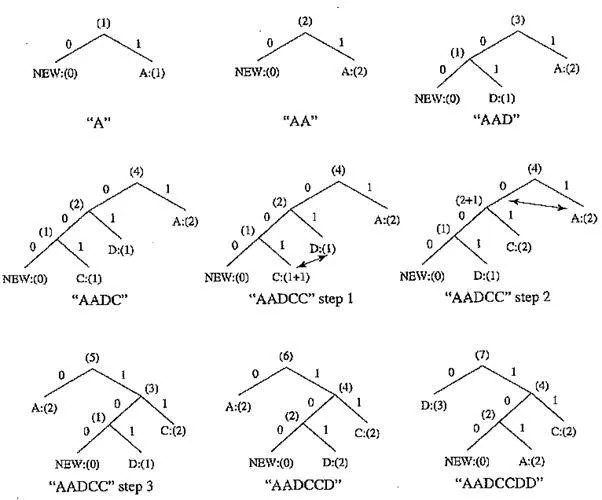
EXAMPLE Adaptive Huffman Coding for Symbol String AADCCDD

Let’s assume that the initial code assignment for both the encoder and decoder simply follows the ASCII order for the 26 symbols in an alphabet, A through Z, as the following table shows. To improve the implementation of the algorithm, we adopt an additional rule: if any character/symbol is to be sent the first time, it must be preceded by a special symbol, NEW. The initial code for NEW is 0. The count for NEW is always kept as 0 (the count is never increased); hence it is always denoted as NEW:(0) in the following figure.

The following figure shows the Huffman tree after each step. Initially, there is no tree. For the first A, 0 for NEW and the initial code 00001 for A are sent. Afterward, the tree is built and shown as the first one, labeled A. Now both the encoder and decoder have constructed the same first tree, from which it can be seen that the code for the second A is 1. The code sent is thus 1.

After the second A, the tree is updated, shown labeled as AA. The updates after receiving D and C are similar. More subtrees are spawned, and the code for NEW is getting longer — from 0 to 00 to 000.

Table Initial code assignment for AADCCDD using adaptive Huffman coding

Adaptive Huffman tree for AADCCDD

From AADC to AADCC takes two swaps. To illustrate the update process clearly, this is shown in three steps, with the required swaps again indicated by arrows.

·         AADCC Step 1. The frequency count for C is increased from 1 to 1 + 1 = 2; this necessitates its swap with D:(l).

·         AADCC Step 2. After the swap between C and D, the count of the parent node of C : (2) will be increased from 2 to 2 + 1 = 3; this requires its swap with A : (2).

AADCC Step 3. The swap between A and the parent of C is completed.

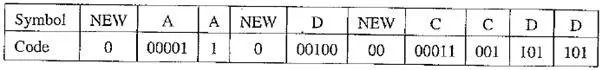
Table Sequence of symbols and codes sent to the decoder

It is important to emphasize that the code for a particular symbol often changes during the adaptive Huffman coding process. The more frequent the symbol up to the moment, the shorter the code. For example, after AADCCDD, when the character D overtakes A as the most frequent symbol, its code changes from 101 to 0. This is of course fundamental for the adaptive algorithm — codes are reassigned dynamically according to the new probability distribution of the symbols.

The “Squeeze Page” on this book’s web site provides a Java applet for adaptive Huffman coding that should aid you in learning this algorithm.