The Lempel – Ziv – Welch (LZW) algorithm employs an adaptive, dictionary – based compression technique. Unlike variable – length coding, in which the lengths of the codewords are different, LZW uses fixed – length codewords to represent variable – length strings of symbols / characters that commonly occur together, such as words in English text.

As in the other adaptive compression techniques, the LZW encoder and decoder builds up the same dictionary dynamically while receiving the data — the encoder and the decoder both develop the same dictionary. Since a single code can now represent more than one symbol / character, data compression is realized.

LZW proceeds by placing longer and longer repeated entries into a dictionary, then emitting the code for an element rather than the string itself, if the element has already been placed in the dictionary. The predecessors of LZW are LZ77 and LZ78, due to Jacob Ziv and Abraham Lempel in 1977 and 1978. Terry Welch improved the technique in 1984. LZW is used in many applications, such as UNIX compress, GIF for images, V.42 bis for modems, and others.

ALGORITHM LZW COMPRESSION

EXAMPLE LZW Compression for String ABABBABCABABBA

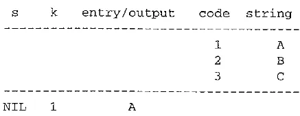
Let’s start with a very simple dictionary (also referred to as a string table), initially containing only three characters, with codes as follows:

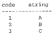
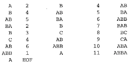
Now if the input string is ABABBABCABABBA, the LZW compression algorithm works as follows:

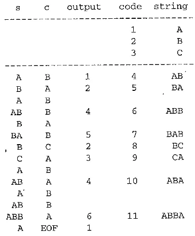
The output codes are 124523461. Instead of 14 characters, only 9 codes need to be sent. If we assume each character or code is transmitted as a byte, that is quite a saving (the compression ratio would be 14 / 9 — 1.56). (Remember, the LZW is an adaptive algorithm, in which the encoder and decoder independently build their own string tables. Hence, there is no overhead involving transmitting the string table.)

Obviously, for our illustration the above example is replete with a great deal of redundancy in the input string, which is why it achieves compression so quickly. In general, savings for LZW would not come until the text is more than a few hundred bytes long.

The above LZW algorithm is simple, and it makes no effort in selecting optimal new strings to enter into its dictionary. As a result, its string table grows rapidly, as illustrated above. A typical LZW implementation for textual data uses a 12 – bit codelength. Hence, its dictionary can contain up to 4,096 entries, with the first 256 (0 – 255) entries being ASCII codes. If we take this into account, the above compression ratio is reduced to (14 x 8) / (9 x 12) = 1.04.

ALGORITHM LZW DECOMPRESSION (SIMPLE VERSION)

EXAMPLE LZW decompression for string ABABBABCABABBA

Input codes to the decoder are 124523461. The initial string table is identical to what is used by the encoder.

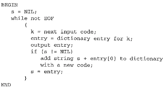
The LZW decompression algorithm then works as follows:

Apparently the output string is ABABB ABC ABABB A — a truly lossless result!

LZW Algorithm DetailsA more careful examination of the above simple version of the LZW decompression algorithm will reveal a potential problem. In adaptively updating the dictionaries, the encoder is sometimes ahead of the decoder. For example, after the sequence ABABB, the encoder will output code 4 and create a dictionary entry with code 6 for the new string ABB.

On the decoder side, after receiving the code 4, the output will be AB, and the dictionary is updated with code 5 for a new string, BA. This occurs several times in the above example, such as after the encoder outputs another code 4, code 6. In a way, this is anticipated — after all, it is a sequential process, and the encoder had to be ahead. In this example, this did not cause problem.

Welch points out that the simple version of the LZW decompression algorithm will break down when the following scenario occurs. Assume that the input string is ABAB – BABCABBABBAX….

The LZW encoder:

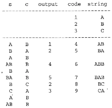
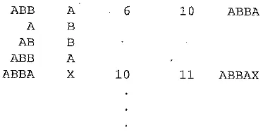
The sequence of output codes from the encoder (and hence the input codes for the decoder) is 24523 6 10…..

The simple LZW decoder:

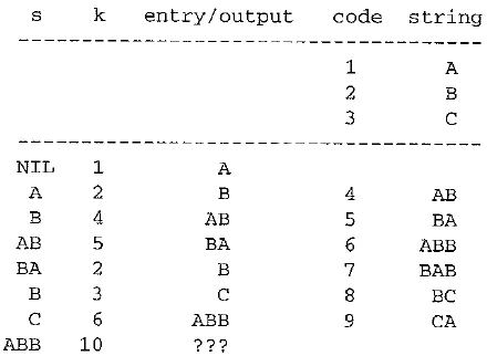
“???” indicates that the decoder has encountered a difficulty: no dictionary entry exists for the last input code, 10. A closer examination reveals that code 10 was most recently created at the encoder side, formed by a concatenation of Character, String, Character. In this case, the character is A, and string is BB — that is, A + BB + A. Meanwhile, the sequence of the output symbols from the encoder are A, BB, A, BB, A.

This example illustrates that whenever the sequence of symbols to be coded is Character, String, Character, String, Character, and so on, the encoder will create a new code to represent Character + String + Character and use it right away, before the decoder has had a chance to create it!

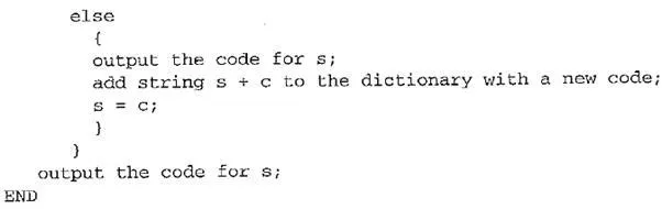
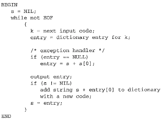
Fortunately, this is the only case in which the above simple LZW decompression algorithm will fail. Also, when this occurs, the variable s — Character + String. A modified version of the algorithm can handle this exceptional case by checking whether the input code has been defined in the decoder’s dictionary. If not, it will simply assume that the code represents the symbols s + s[0]; that is Character + String + Character.

ALGORITHM LZW DECOMPRESSION (MODIFIED)

Implementation requires some practical limit for the dictionary size — for example, a maximum of 4,096 entries for GIF and 2,048 entries for V.42 bis. Nevertheless, this still yields a 12 – bit or 11 – bit code length for LZW codes, which is longer than the word length for the original data — 8 – bit for ASCII.

In real applications, the code length / is kept in the range of [l0 – lmax] For the UNIX compress command, l0 = 9 and lmax is by default 16. The dictionary initially has a size of 2l°. When it is filled up, the code length will be increased by 1; this is allowed to repeat

l = lmax

If the data to be compressed lacks any repetitive structure, the chance of using the new codes in the dictionary entries could be low. Sometimes, this will lead to data expansion instead of data reduction, since the code length is often longer than the word length of the original data. To deal with this, V.42 bis, for example, has built in two modes: compressed and transparent. The latter turns off compression and is invoked when data expansion is detected.

Since the dictionary has a maximum size, once it reaches 2lmas entries, LZW loses its adaptive power and becomes a static, dictionary – based technique. UNIX compress, for example, will monitor its own performance at this point. It will simply flush and reinitialize the dictionary when the compression ratio falls below a threshold. A better dictionary management is perhaps to remove the LRU (least recently used) entries. V.42 bis will look for any entry that is not a prefix to any other dictionary entry, because this indicates that the code has not been used since its creation.