One of the most commonly used compression techniques in multimedia data compression is differential coding. The basis of data reduction in differential coding is the redundancy in consecutive symbols in a datastream. When we examined how audio must be dealt with via subtraction from predicted values. Audio is a signal indexed by one dimension, time. Here we consider how to apply the lessons learned from audio to the context of digital image signals that are indexed by two, spatial, dimensions (x, y).
Differential Coding of Images
Let’s consider differential coding in the context of digital images. In a sense, we move from signals with domain in one dimension to signals indexed by numbers in two dimensions (x, y) — the rows and columns of an image. Later, we’ll look at video signals. These are even more complex, in that they are indexed by space and time (x, y, t).
Because of the continuity of the physical world, the gray – level intensities (or color) of background and foreground objects in images tend to change relatively slowly across the image frame. Since we were dealing with signals in the time domain for audio, practitioners generally refer to images as signals in the spatial domain. The generally slowly changing nature of image spatially produces a high likelihood that neighboring pixels will have similar intensity values. Given an original image I (x, y), using a simple difference operator we can define a difference image d(x, y) as follows:
d [x , y) = l {x , y) – l (x – 1, y)
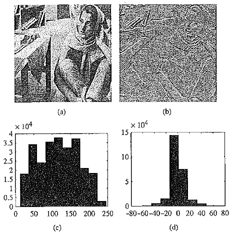
Distributions for original versus derivative images. (a , b) original gray – level image and its partial derivative image; (c,d) histograms for original and derivative images. This figure uses a commonly employed image called Barb
This is a simple approximation of a partial differential operator δ / δ x applied to an image defined in terms of integer values of x and y.
Another approach is to use the discrete version of the 2D Laplacian operator to define a difference image d(x, y) as
d {x, y) = 4 / (.v, y) – I (x, y – 1) – I (x, y + 1) – I (x + 1, y) – I (x – 1, y)
In both cases, the difference image will have a histogram as in the above figure (d), derived from the d(x, y) partial derivative image in (b) for the original image in (a). Notice that the histogram for I is much broader, as in (c). It can be shown that image I has larger entropy than image d, since it has a more even distribution in its intensity values. Consequently, Huffman coding or some other variable – length coding scheme will produce shorter bit – length codewords for the difference image. Compression will work better on a difference image.
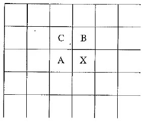
Neighboring pixels for predictors in lossless JPEG. Note that any of A, B, or C has already been decoded before it is used in the predictor, on the decoder side of an encode / decode cycle
Lossless JPEG
Lossless JPEG is a special case of the JPEG image compression. It differs drastically from other JPEG modes in that the algorithm has no lossy steps. Lossless JPEG is invoked when the user selects a 100% quality factor in an image tool. Essentially, lossless JPEG is included in the JPEG compression standard simply for completeness.
The following predictive method is applied on the unprocessed original image (or each color band of the original color image). It essentially involves two steps: forming a differential prediction and encoding.
A predictor combines the values of up to three neighboring pixels as the predicted value for the current pixel, indicated by X in the above figure. The predictor can use any one of the seven schemes listed in the following table. If predictor PI is used, the neighboring intensity value A will be adopted as the predicted intensity of the current pixel; if
Table Predictors for lossless JPEG
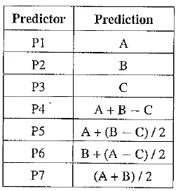
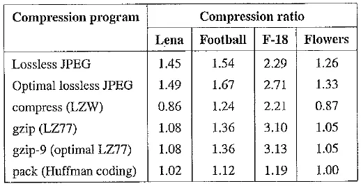
Table Comparison of lossless JPEG with other lossless compression programs
predictor P4 is used, the current pixel value is derived from the three neighboring pixels as A + B — C; and so on.
The encoder compares the prediction with the actual pixel value at position X andencodes the difference using one of the lossless compression techniques we have discussed, such as the Huffman coding scheme.
Since prediction must be based on previously encoded neighbors, the very first pixel in the image 1(0, 0) will have to simply use its own value. The pixels in the first row always use predictor PI, and those in the first column always use P2.
Lossless JPEG usually yields a relatively low compression ratio, which renders it impractical for most multimedia applications. An empirical comparison using some 20 images indicates that the compression ratio for lossless JPEG with any one of the seven predictors ranges from 1.0 to 3.0, with an average of around 2.0. Predictors 4 to 7 that consider neighboring nodes in both horizontal and vertical dimensions offer slightly better compression (approximately 0.2 to 0.5 higher) than predictors 1 to 3.
Table shows a comparison of the compression ratio for several lossless compression techniques using test images Lena, football, F – 18, and flowers. These standard images used for many purposes in imaging work are shown on the textbook web site in the Further Exploration section for this chapter.
This chapter has been devoted to the discussion of lossless compression algorithms. It should be apparent that their compression ratio is generally limited (with a maximum at about 2 to 3). However, many of the multimedia applications we will address in the next several chapters require a much higher compression ratio. This is accomplished by lossy compression schemes.