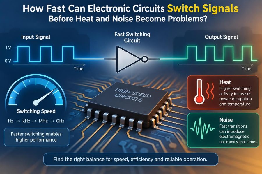

A phone camera captures a fast-moving scene, a motor controller corrects its current, and a data link sends billions of bits every second. All depend on electronic circuits changing state quickly enough to make a useful decision before the world has moved on.
It is tempting to ask for one maximum switching speed. In practice, no universal limit exists. A tiny logic gate may toggle extraordinarily fast, while the board, package, power supply, cables, and load turn that same transition into a heating, timing, or interference problem.
The challenge becomes visible when a design that worked at a low clock rate suddenly runs hot, produces erratic measurements, fails an electromagnetic-compatibility test, or communicates unreliably. The signal may still look like a neat square wave at its source, but it no longer behaves that way at its destination.
Fast switching is therefore not simply about making edges faster. It is about controlling energy, current paths, timing, and unwanted radiation well enough that the circuit can use speed without being defeated by it.
⚡ Switching Speed Means More Than Clock Frequency
A circuit can switch “fast” in two related but different ways: it can repeat events frequently, or it can make each transition rapidly. Clock frequency counts repeated cycles per second. Rise time and fall time describe how long a voltage takes to move between logic levels.
A 10 MHz clock with a 1 ns edge can create many of the same signal-integrity concerns as a much faster clock with slow edges. Interconnects react mainly to edge rate, because a sharp edge contains substantial high-frequency content.
📏 The Useful Time Scales
Period, rise time, propagation delay, and settling time answer different design questions. The period says how much time a complete cycle occupies. Propagation delay says when a change arrives at another point. Settling time says when an analog or digital node has become reliably quiet enough to use.
For a digital receiver, the relevant question is not merely “did voltage change?” It is “was the required logic level present and stable during the receiver’s sampling window?”
🌊 Why a Square Wave Is Never Truly Square
An ideal square wave changes voltage instantly and contains unlimited harmonics. Real drivers have finite current, so their edges slope. Real traces, packages, and probes also add resistance, inductance, and capacitance that reshape the waveform.
The finite edge is helpful in one sense: it limits bandwidth. But if the edge is too slow, the receiver spends longer near its threshold, where noise can cause uncertainty. If it is too fast, ringing and radiation become more difficult to manage.
🧮 Edge Rate Sets the Bandwidth Burden
A useful engineering rule estimates a signal’s bandwidth from rise time rather than repetition rate: bandwidth ≈ 0.35 / rise time for a common first-order approximation. A 1 ns rise time therefore demands attention well into the hundreds of megahertz, even if the bit rate is modest.
This is an estimate, not a complete model. Driver shape, allowable distortion, and receiver behavior matter. Its value is practical: it warns designers not to treat a slow-looking digital clock as a low-frequency problem when its edges are sharp.
🔋 Every Transition Moves Energy
Most switching heat comes from repeatedly charging and discharging capacitance. That capacitance includes transistor gates, IC pins, PCB traces, cable conductors, and the input capacitance of connected devices.
For a capacitive load, the energy drawn from the supply on a 0-to-V transition is approximately C × V². Repeating that event at frequency f produces the familiar dynamic-power estimate: P ≈ C × V² × f.
This explains why higher activity, higher voltage, larger loads, and faster clocks can all raise power dissipation. It also explains why reducing supply voltage is often a powerful lever, although it may reduce noise margin or require a different process technology.
🔥 Where the Heat Actually Goes
In an ideal CMOS output charging a capacitor, energy is temporarily stored in the capacitor and then largely dissipated during discharge. In real circuits, additional loss occurs in transistor resistance, package leads, traces, termination networks, and power-conversion components.
A power transistor may also dissipate considerable energy while both its voltage and current are high during a transition. This is especially significant in switching converters, inverters, and motor drives, where switching a load is not equivalent to toggling a tiny logic input.
🚦 CMOS, Bipolar, and Power-Switching Limits
Logic families and power devices reach speed limits for different reasons. CMOS logic is often dominated by charging capacitance and internal transistor delay. Bipolar circuits can switch very quickly but may consume substantial static power. Power MOSFETs and IGBTs must move much more charge and handle far more energy per event.
The best device is therefore application-specific. A fast gate driver that is excellent for a small MOSFET may produce unacceptable overshoot and loss when paired with a large power module and a long current loop.
🧲 Inductance Fights Rapid Current Change
Inductance resists a changing current according to V = L × di/dt. When a switch turns current off rapidly, even a small parasitic inductance in leads or traces can generate a significant voltage spike.
That spike can overstress a semiconductor, create ringing, or inject noise into nearby circuits. The issue is not limited to coils: every physical current loop has some inductance, including the loop formed by a transistor, decoupling capacitor, and return path.
🪣 Capacitance Demands Peak Current
Capacitance resists a changing voltage according to I = C × dV/dt. A faster voltage edge into the same capacitance requires more instantaneous current from the driver.
This is why an IC output may seem fast when unloaded but slow noticeably when connected to several inputs, a long trace, or a measurement probe. It is also why gate drivers for power MOSFETs are designed to source and sink high peak currents, even when their average power is modest.
🔁 Ringing Is Energy Moving Back and Forth
When inductance and capacitance are connected, they can exchange energy and oscillate. A fast edge excites this resonance, creating overshoot, undershoot, and ringing. Resistance eventually damps the motion, but not necessarily before a receiver misreads the signal or a device exceeds its rating.
Ringing is not always a sign that the nominal clock frequency is too high. Often it indicates a mismatch between edge speed, interconnect geometry, and termination.
🛣️ A PCB Trace Can Behave Like a Transmission Line
A trace behaves as a transmission line when the edge travels a meaningful distance before the transition is complete. In that situation, voltage and current are distributed along the trace rather than changing everywhere at once.
The familiar rule of thumb is to investigate transmission-line behavior when trace flight time becomes an appreciable fraction of rise time. The exact threshold depends on allowable error, but waiting for obvious failure is not a sound strategy.
📡 Reflections Distort the Receiving End
A wave reaching a discontinuity—such as an unterminated input, connector, branch, or impedance change—partly reflects. The reflected wave can combine with the original signal and create a doubled-looking step, ringing, or a delayed threshold crossing.
A short trace can still have reflections if the driver edge is very fast. Conversely, a long trace with deliberately controlled, slower edges can be easier to manage.
🧩 Termination Trades Signal Cleanliness for Power or Delay
Termination controls reflections by making the signal path look more like its characteristic impedance. Series termination near the driver is efficient for point-to-point links because it limits the launched wave without creating continuous DC current.
Parallel termination at the receiver can give a clean endpoint but may consume static power. AC termination can reduce that DC loss, though its behavior depends on frequency and startup conditions. The choice should follow topology, data rate, duty cycle, and power budget.
🌐 Return Paths Matter as Much as Signal Paths
High-frequency current returns along the path of least impedance, usually close to the signal trace through a reference plane. It does not necessarily return by the geometrically shortest route.
A split in the reference plane, a poorly placed connector, or a signal routed over a gap forces return current to spread out. That enlarges the loop, increasing inductance, radiation, and susceptibility to external noise.
📣 Fast Edges Create Electromagnetic Interference
Any changing current loop can radiate, and any changing electric field can couple into another conductor. Faster transitions increase the frequency range over which these mechanisms matter. Long traces, cable assemblies, and poorly contained return paths make particularly effective unintended antennas.
Electromagnetic interference, or EMI, is not solved by shielding alone. A shield can help, but reducing loop area, controlling return paths, and avoiding unnecessary edge speed often address the source more directly.
🎚️ Noise Margin Is the Receiver’s Safety Space
Digital logic does not require a perfectly clean voltage; it requires sufficient separation between guaranteed output levels and recognized input thresholds. That separation is the noise margin.
Supply bounce, crosstalk, ringing, temperature variation, and process variation all spend part of this margin. A design that works on one bench at room temperature may have little remaining margin across its operating range.
🗣️ Crosstalk Lets One Signal Disturb Another
Adjacent traces couple through electric and magnetic fields. A rapidly changing “aggressor” trace can induce a pulse on a nearby “victim” trace. The effect depends on spacing, parallel run length, layer stackup, termination, and edge rate.
Clock lines, resets, analog inputs, and high-impedance control nodes deserve special routing attention. Spacing helps, but a continuous reference plane and a sensible layer arrangement are often equally important.
🏔️ Ground Bounce Moves the Local Reference
“Ground” is not an ideal zero-volt point during a fast transient. Current flowing through package and PCB inductance develops voltage, so the local ground at an IC can move relative to ground elsewhere.
When multiple outputs switch together, this ground bounce can shift input thresholds and corrupt quiet signals. The companion problem on the positive rail is supply droop or bounce. Both are consequences of a power-distribution network that cannot deliver transient current cleanly enough.
🔌 Decoupling Capacitors Supply the First Burst
Decoupling capacitors placed near IC power pins provide local charge during fast switching events. Their effectiveness depends on more than capacitance value: mounting inductance, package type, plane geometry, and frequency behavior matter greatly.
A distant bulk capacitor can support slower load changes but cannot replace close, low-inductance decoupling. Good power integrity uses layers of support: local capacitors for fast demand, broader plane capacitance, and regulators or bulk storage for slower energy replenishment.
🌡️ Temperature Changes Electrical Behavior
As a device warms, resistance, leakage, timing, and switching characteristics can shift. Heat also raises the difficulty of removing further heat, because the temperature difference available to the surroundings shrinks.
This can create a feedback loop: more loss raises temperature, and altered parameters may raise loss further. Designers use thermal models and measurements to check worst-case operating conditions rather than assuming room-temperature bench results will scale safely.
⏱️ Timing Closure Is a System Problem
At high digital speeds, a path budget includes clock uncertainty, source delay, trace delay, receiver setup time, hold time, and variation. A logic gate can be fast enough in isolation while the complete path still fails timing.
Clock distribution deserves particular care. Skew—different clock arrival times at different receivers—can reduce useful timing margin even if every individual waveform looks clean.
📈 Analog Circuits Have a Different Kind of Speed Limit
Analog amplifiers and comparators are constrained by bandwidth, slew rate, settling behavior, stability, and noise. A high slew rate means an output can move quickly, but it does not guarantee that the final value is accurate or free from overshoot.
For an analog-to-digital converter, the front-end amplifier must settle within the required error band before sampling. “Fast enough” is therefore tied to resolution and accuracy, not only to the sample rate.
🛠️ Power Converters Show the Classic Trade-Off
Increasing a switching converter’s frequency can reduce the size of inductors and capacitors, which is attractive in compact products. But each switching event has loss, and magnetic components, gate drive, layout parasitics, and EMI all become more demanding.
Lower frequency may improve switching efficiency but require larger energy-storage components and can move audible effects into an inconvenient range. There is no automatic winner; the useful choice balances efficiency, size, transient response, thermal limits, and emissions.
🚗 Motor Drives Add Cable and Load Effects
In a motor inverter, fast voltage edges can improve switching loss but can also cause reflected-wave overvoltage at the motor, especially with long cables. Motor winding insulation, bearing currents, common-mode noise, and conducted emissions may become concerns.
Gate resistors, output filters, controlled slew-rate drivers, and appropriate cable practices can be more effective than simply choosing the fastest possible transistor driver.
🔬 Measurement Can Create a False Problem
A probe’s capacitance can slow a sensitive node, while a long oscilloscope ground clip forms an inductive loop that readily picks up ringing. The displayed waveform may then exaggerate noise that is not actually present at the device pins.
Use a short ground spring or a suitable differential probe for fast measurements. Check probe bandwidth, sampling method, and probing location before redesigning hardware around a suspicious trace.
🧪 Simulate Early, Then Measure the Real Hardware
SPICE models, field-solvers, and power-integrity tools can expose likely trouble before a board is built. They are most useful when component models, stackup data, and parasitic assumptions are realistic.
Simulation is not a substitute for measurement. Actual packages, connectors, assembly variation, and loads can differ from models. A sound workflow uses simulation to narrow decisions, then validates the completed system under realistic voltage, temperature, and activity conditions.
🧱 Layout Choices That Preserve Speed
Good high-speed layout is mostly deliberate current-path design. Keep switching loops compact, place decoupling capacitors directly between power and ground paths, maintain solid reference planes, and avoid stubs on sensitive nets.
- Route fast signals over an uninterrupted reference plane.
- Keep differential pairs coupled and avoid unnecessary asymmetry.
- Separate noisy power-switching loops from low-level analog sensing.
- Place series resistors close to the driving pin when they are used for edge control.
- Provide short, wide paths for high transient current.
These practices are not cosmetic rules. Each reduces unwanted inductance, impedance discontinuity, or coupling path.
🧯 Slowing an Edge Can Be the Correct Fix
Designers sometimes treat a slower edge as a performance failure. If the receiver still meets setup and hold requirements, a controlled slower edge can reduce overshoot, EMI, crosstalk, and stress on components.
Series resistance, selectable drive strength, gate resistors, and slew-rate-controlled drivers are common tools. The goal is not maximum edge rate; it is the fastest transition that meets timing while remaining electrically well behaved.
⚠️ Common Speed-Related Design Mistakes
- Designing from clock rate alone: edge rate, not only repetition rate, determines many interconnect problems.
- Adding capacitors without considering inductance: placement and loop geometry can matter more than a larger nominal value.
- Using a ground trace instead of a reference plane: the return path becomes higher impedance and less predictable.
- Ignoring simultaneous switching: several outputs changing together can be much worse than one channel on a bench.
- Fixing a waveform only at the source: verify what the receiver sees at its pins.
🧭 A Practical Way to Set a Switching-Speed Target
Start from system requirements: data throughput, control-loop bandwidth, conversion accuracy, and permitted latency. Then establish the timing budget, load capacitance or current, interconnect length, voltage ratings, thermal path, and emissions constraints.
Next, choose a realistic edge-rate target rather than accepting the strongest available driver by default. Prototype critical paths, inspect waveforms at the receiver, measure temperature and supply noise, and test across credible operating conditions. This process turns “how fast?” into an evidence-based engineering decision.
✅ The Core Principle: Fast Enough, Not Fastest
Electronic circuits do not encounter one abrupt speed wall. Their usable switching rate is bounded by a set of interacting limits: device delay, capacitive energy, inductive voltage, interconnect reflections, power integrity, thermal resistance, receiver margin, and electromagnetic emissions.
A successful design recognizes which limit dominates in its application. A microprocessor board may be constrained by timing and signal integrity; a converter by switching loss and EMI; a motor drive by voltage overshoot and insulation stress. The remedy follows the mechanism, not a generic instruction to speed up or slow down.
The best switching speed is the one that meets functional timing with controlled heat, clean power, adequate noise margin, and manageable emissions. That balance is what lets a circuit remain reliable beyond the ideal conditions of a first test bench. 🔌⚡🛠️