Introduction

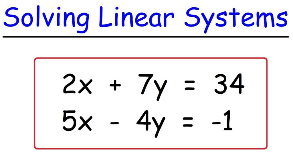
The necessity to solve linear systems of equations is commonplace in numerical computing. This chapter considers a few examples of how such problems arise (more examples will be seen in subsequent chapters) and the numerical problems that are frequently associated with attempts to solve them. We are particularly interested in the phenomenon of ill conditioning. We will largely concentrate on how the problem arises, what its effects are, and how to test for this problem.1 In addition to this, we will also consider methods of solving linear systems other than the Gaussian elimination method that you most likely learned in an elementary linear algebra course. More specifically, we consider LU and QR matrix factorization methods, and iterative methods of linear system solution. The concept of a singular value decomposition (SVD) is also introduced.

We will often employ the term “linear systems” instead of the longer phrase “linear systems of equations.” However, the reader must be warned that the phrase “linear systems” can have a different meaning from our present usage. In signals and systems courses you will most likely see that a “linear system” is either a continuous-time (i.e., analog) or discrete-time (i.e., digital) dynamic system whose input/output (I/O) behavior satisfies superposition. However, such dynamic systems can be described in terms of linear systems of equations.

Least-Squares Approximation And Linear Systems