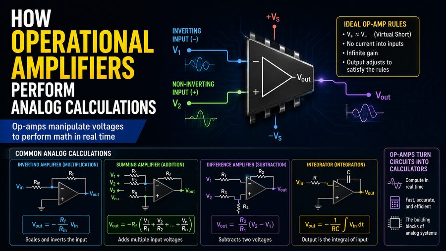

Long before modern digital computers became dominant, engineers built machines that could solve mathematical problems using continuous electrical signals instead of binary numbers. At the heart of many of these analog computing systems was a deceptively simple electronic component: the operational amplifier, commonly called an op-amp. 🔌🧠
An operational amplifier is a high-gain electronic amplifier with two input terminals and one output terminal. By combining an op-amp with resistors, capacitors, and feedback networks, engineers can make circuits that perform mathematical operations such as:
- Addition
- Subtraction
- Multiplication by a constant
- Integration
- Differentiation
- Averaging
- Comparison
- Filtering
This ability to manipulate voltages according to mathematical relationships is the reason the device is called an operational amplifier: it was originally developed to perform mathematical operations in analog computers.
🔬 What Is an Operational Amplifier?
An op-amp typically has two inputs:
- The non-inverting input, marked
+ - The inverting input, marked
−
It also has an output.
The basic behavior can be described approximately as:
Output voltage = gain × (non-inverting input voltage − inverting input voltage)
Mathematically:
Vout = A(V+ − V−)
where:
Voutis the output voltageAis the open-loop gainV+is the voltage at the non-inverting inputV−is the voltage at the inverting input
The open-loop gain of an op-amp is extremely large, often tens or hundreds of thousands or more.
Because the gain is so high, even a very small difference between the two inputs can drive the output strongly positive or negative.
By itself, this enormous gain is difficult to control. The real power of op-amps appears when engineers use negative feedback. 🔄
🔁 Why Negative Feedback Is So Important
Negative feedback means sending some of the output signal back toward the inverting input.
This causes the circuit to continuously correct itself.
In a properly operating closed-loop circuit, the op-amp adjusts its output so that the difference between its two input voltages becomes extremely small.
Engineers often use the useful approximation:
V+ ≈ V−
This is sometimes called the virtual short principle.
The inputs are not physically shorted together. Instead, the high gain and feedback cause their voltages to become nearly equal.
Another common ideal approximation is that almost no current flows into the op-amp’s input terminals.
These two assumptions make many op-amp circuits surprisingly easy to analyze mathematically.
➗ The Inverting Amplifier: Multiplying by a Constant
One of the simplest op-amp calculations is multiplication by a fixed number.
Consider an inverting amplifier.
A signal enters the inverting input through resistor Rin, while another resistor Rf connects the output back to the same input.
The voltage gain is approximately:
Vout = −(Rf / Rin) × Vin
The ratio of the resistors determines the multiplication factor.
For example, suppose:
Rin = 10 kΩ
and:
Rf = 20 kΩ
Then:
Rf / Rin = 2
So:
Vout = −2Vin
If the input is:
Vin = 1 V
the output becomes approximately:
Vout = −2 V
The circuit has therefore multiplied the input voltage by −2.
The minus sign means that the signal is inverted.
This is a genuine analog mathematical calculation performed continuously by electrical voltages. ⚡
➕ How an Op-Amp Adds Several Signals
An op-amp can also act as an analog adder.
A common design is called a summing amplifier.
Multiple input voltages are each connected to the inverting input through separate resistors.
The op-amp combines the currents produced by these inputs.
For equal input resistors, the output can be proportional to:
Vout = −(V1 + V2 + V3 + …)
For example, suppose three input voltages are:
V1 = 1 V
V2 = 2 V
V3 = 0.5 V
A properly designed summing amplifier might produce:
Vout = −3.5 V
If another amplifier inverts the result again, the final output could be:
+3.5 V
This kind of circuit was extremely useful in analog computers because many physical equations require several quantities to be added together.
Summing amplifiers are also used in audio mixing, sensor interfaces, and control systems. 🎚️
➖ Performing Subtraction
Op-amps can also subtract one voltage from another.
A difference amplifier produces an output proportional to the difference between two input signals.
Conceptually:
Vout = K(V2 − V1)
where K is a gain determined by resistor values.
Suppose:
V1 = 2 V
and:
V2 = 5 V
If the gain is 1:
Vout = 3 V
This makes difference amplifiers useful for measuring small voltage differences in circuits where both signals may share a common background voltage.
They are especially important in sensor systems and measurement electronics.
📊 Weighted Addition
The inputs of a summing amplifier do not all need to contribute equally.
Different resistor values can assign different weights to each signal.
For example, a circuit could calculate something equivalent to:
Vout = −(2V1 + 0.5V2 + 3V3)
This allows an op-amp to implement a weighted sum.
Weighted sums appear throughout engineering mathematics.
They are used in:
- Control systems
- Signal processing
- Audio electronics
- Sensor fusion
- Analog computing
- Neural-network-inspired circuits
In this sense, a carefully designed resistor network acts almost like the coefficients in an equation. 🧮
∫ How Op-Amps Perform Integration
One of the most impressive analog calculations performed by op-amps is integration.
In mathematics, integration accumulates a quantity over time.
An op-amp integrator typically uses:
- A resistor at the input
- A capacitor in the feedback path
The output is approximately proportional to the time integral of the input:
Vout = −(1/RC) ∫ Vin dt
where:
Ris resistanceCis capacitanceVinis the input voltage
Imagine applying a constant positive voltage to an integrator.
The capacitor gradually charges, causing the output voltage to change steadily over time.
A constant input can therefore produce a ramp-shaped output.
For example:
Constant input ➡️ Linearly changing output
This behavior directly represents mathematical integration.
🚗 Why Integration Matters in Physical Systems
Integration appears constantly in physics.
Velocity is the integral of acceleration:
Velocity = ∫ acceleration dt
Position is the integral of velocity:
Position = ∫ velocity dt
An analog computer could therefore represent acceleration as a voltage, send that voltage into an integrator to calculate velocity, and then integrate again to calculate position.
Conceptually:
Acceleration voltage ➡️ Integrator ➡️ Velocity voltage ➡️ Integrator ➡️ Position voltage
This allowed early analog computers to model aircraft motion, missile trajectories, mechanical systems, and other continuously changing processes. ✈️📈
d/dt How Op-Amps Perform Differentiation
The mathematical opposite of integration is differentiation.
A differentiator produces an output proportional to how quickly the input voltage changes.
A simplified op-amp differentiator uses:
- A capacitor in the input path
- A resistor in the feedback path
Its output behaves approximately like:
Vout = −RC × dVin/dt
If the input voltage changes very quickly, the output becomes large.
If the input remains constant, its derivative is zero, so the output approaches zero.
For example:
Constant voltage ➡️ Approximately zero output
Rapid voltage change ➡️ Large output pulse
Differentiators can therefore detect edges, transitions, and rapid signal changes.
📉 Why Practical Differentiators Need Careful Design
Ideal differentiators strongly amplify high-frequency signals.
Unfortunately, electronic noise often contains high-frequency components.
Therefore, a perfect mathematical differentiator would also amplify unwanted noise.
Practical differentiator circuits usually include additional resistors or capacitors to limit their frequency response.
This illustrates an important difference between mathematical equations and real electronics: physical circuits have limitations.
Engineers must account for:
- Noise
- Component tolerances
- Frequency response
- Power supply limits
- Op-amp bandwidth
- Stability
⚖️ Averaging Signals
An op-amp can also calculate an average.
Suppose three signals enter a summing amplifier.
If the circuit first adds:
V1 + V2 + V3
and then multiplies the result by:
1/3
the output becomes:
(V1 + V2 + V3) / 3
That is the arithmetic mean.
Analog averaging can be useful when combining measurements from multiple sensors or smoothing signals.
🔄 Scaling and Unit Conversion
Op-amps frequently perform scaling calculations.
Suppose a temperature sensor generates:
10 millivolts per degree Celsius
A 50°C measurement would produce:
0.5 V
An op-amp with a gain of 5 could convert this into:
2.5 V
This makes the signal easier for another circuit to process.
Scaling circuits are common between sensors and:
- Analog-to-digital converters
- Microcontrollers
- Industrial controllers
- Measurement instruments
🎛️ Analog Computers and Differential Equations
The real power of op-amp calculations appears when multiple circuits are connected together.
Many physical systems can be described using differential equations.
For example, the movement of a spring-and-mass system depends on relationships between:
- Position
- Velocity
- Acceleration
- Mass
- Spring force
- Damping
Using integrators, summers, and amplifiers, an analog computer can create an electrical network whose voltages obey the same mathematics as the mechanical system.
Instead of calculating one numerical step after another, the analog computer allows voltages to evolve continuously.
The electrical circuit effectively becomes a physical model of the equation. 🧠⚡
🎚️ Op-Amps as Analog Filters
Op-amps are also widely used to build active filters.
Filters perform mathematical operations on signals based on frequency.
Common types include:
- Low-pass filters
- High-pass filters
- Band-pass filters
- Band-stop filters
A low-pass filter allows slow signal variations to pass while reducing rapid fluctuations.
A high-pass filter does the opposite.
These circuits can be viewed as analog mathematical systems because they transform signals according to equations involving frequency and time.
Active filters appear in:
- Audio equipment
- Communication systems
- Sensors
- Medical electronics
- Instrumentation
🔊 Audio Mixing as Analog Arithmetic
Audio mixing provides a practical example of op-amp mathematics.
Suppose a mixing console receives signals from:
- A microphone
- A guitar
- A keyboard
- A music player
A summing amplifier can mathematically add these voltages.
Potentiometers can adjust how strongly each signal contributes.
Conceptually:
Output = a × microphone + b × guitar + c × keyboard + d × music
The coefficients a, b, c, and d correspond to volume settings.
The resulting output is literally an analog weighted sum of several signals. 🎵
⚙️ Real Op-Amps Are Not Perfect
Textbook calculations often treat op-amps as ideal devices.
A perfect op-amp would have:
- Infinite open-loop gain
- Infinite input impedance
- Zero output impedance
- Unlimited bandwidth
- Zero input offset voltage
- Unlimited output voltage
- Instantaneous response
Real op-amps have limitations.
Important specifications include:
📡 Bandwidth
An op-amp cannot amplify signals equally well at every frequency.
At sufficiently high frequencies, its gain decreases.
⚡ Slew Rate
The output cannot change voltage infinitely fast.
The maximum rate at which the output can change is called the slew rate.
🎯 Input Offset Voltage
Even when both inputs should theoretically be equal, small internal imperfections can create an output error.
🔌 Supply Voltage
The output generally cannot exceed the voltage supplied to the op-amp.
A circuit powered from ±15 V supplies cannot produce an arbitrary 100 V output.
📏 Component Accuracy Affects Calculation Accuracy
An op-amp circuit often relies on resistor and capacitor ratios.
If the components are not exact, the mathematical result will also contain some error.
Suppose an amplifier is designed for a gain of exactly 10.
If resistor tolerances shift the ratio slightly, the actual gain might become:
9.95
or:
10.07
High-precision analog circuits therefore use carefully selected components with tight tolerances.
Temperature changes can also alter component values.
🧮 Analog vs. Digital Calculation
Digital computers represent numbers as binary values and calculate through logical operations.
Analog circuits represent quantities using continuously varying voltages or currents.
For example:
Digital computer: velocity may be stored as a binary number.
Analog computer: velocity may be represented by a voltage.
Analog calculations can happen continuously and in parallel.
Several integrators and summing circuits can operate simultaneously.
Digital systems, however, offer major advantages in:
- Accuracy
- Repeatability
- Storage
- Programmability
- Complex logic
- Noise immunity
This is one reason general-purpose digital computing eventually replaced most traditional analog computers.
🤖 Are Analog Calculations Still Useful Today?
Absolutely.
Even though smartphones and laptops rely primarily on digital processors, the physical world is fundamentally analog.
Real-world quantities such as:
- Sound
- Temperature
- Pressure
- Light intensity
- Acceleration
- Electrical current
vary continuously.
Before these signals enter a digital processor, they often need analog conditioning.
Op-amps may amplify them, subtract offsets, filter noise, or scale their range.
This makes operational amplifiers essential in modern electronics.
🩺 Medical and Scientific Applications
Op-amps are especially important in measurement systems.
Consider an electrocardiogram, or ECG.
The electrical signals produced by the heart are extremely small.
Amplifier circuits must increase these signals while rejecting unwanted interference.
Similar techniques are used in:
- EEG brain-signal measurements
- Industrial sensors
- Strain gauges
- Laboratory equipment
- Precision thermometers
- Chemical measurement instruments
Analog calculations help transform tiny physical signals into useful electrical information. 🩺🔬
⚡ A Simple Example of an Analog Calculation System
Imagine a circuit designed to calculate:
Y = 2A + 3B
where A and B are voltages representing physical measurements.
The system could use:
- 🔌 An amplifier to multiply signal A by 2.
- ⚙️ Another amplifier to multiply signal B by 3.
- ➕ A summing amplifier to add the two results.
- 🔄 An additional inverter if the desired polarity needs correction.
If:
A = 1 V
and:
B = 2 V
then:
Y = 2(1) + 3(2)
Y = 2 + 6
Y = 8 V
The resulting voltage physically represents the answer to the equation.
No binary conversion is required.
🌟 The Bigger Picture
Operational amplifiers perform analog calculations by turning mathematical relationships into electrical relationships.
Resistor ratios can create multiplication or division by constants.
Multiple inputs can be summed.
Difference amplifiers can subtract.
Capacitors combined with feedback allow integration and differentiation.
Entire networks of op-amps can represent complex systems of equations.
The fundamental idea is elegant:
Represent numbers as voltages ➡️ Manipulate those voltages with circuits ➡️ Read the output voltage as the mathematical result
That approach helped give rise to analog computers and remains extremely valuable in modern electronics. ⚡🧠
Today, op-amps are found in audio systems, sensors, medical instruments, industrial controllers, power electronics, laboratory equipment, and countless embedded devices.
Although modern computing is dominated by digital processors, operational amplifiers continue performing analog mathematics quietly inside the circuits that connect those processors to the real world.
In that sense, every op-amp is a tiny mathematical machine—continuously adding, subtracting, scaling, integrating, or filtering electrical signals at the speed of the underlying physics. 🔌📊