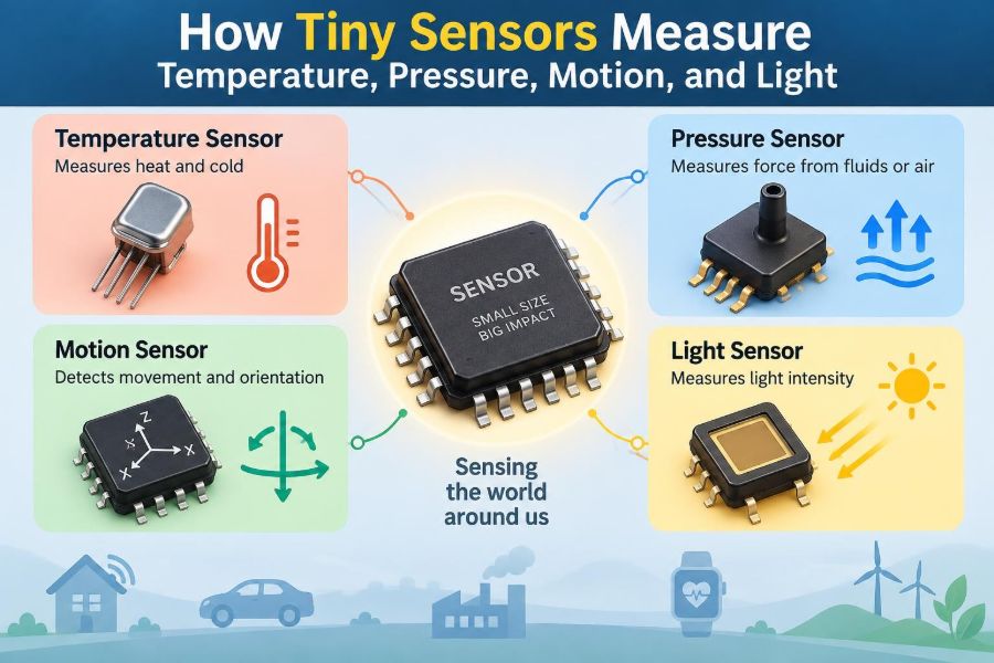

A phone brightens its screen when you step outdoors, a car warns when a tire loses air, and a fitness watch notices that you have started walking. In each case, a tiny electronic device has translated a physical change in the real world into information a circuit can use.
These devices are sensors. They do not “understand” heat, force, movement, or light in the human sense. Instead, they exploit a material property that changes predictably: resistance, voltage, capacitance, charge, frequency, or current.
That conversion is at the heart of modern electronics. A microcontroller can calculate rapidly, but it cannot directly feel the environment. Sensors provide its input—often through structures too small to see without magnification.
Understanding how sensors work makes datasheets easier to read, helps with reliable circuit design, and explains why measurements sometimes drift, lag, or disagree with expectation.
🧭 A Sensor Is a Physical-to-Electrical Translator
A sensor is a device that converts a measurand—the quantity being measured—into an electrical signal. The measurand might be temperature, pressure, acceleration, illumination, humidity, magnetic field, or gas concentration.
The resulting signal is usually a voltage, current, resistance, capacitance, pulse frequency, or digital data word. Electronics can amplify, filter, digitize, store, display, or use that signal to control another device.
A thermostat is a familiar example. Its temperature sensor observes thermal conditions, while the controller compares that reading with a setpoint and decides whether to operate heating or cooling equipment.
🔗 The Measurement Chain Has Several Parts
The sensing element is only the first part of a useful measurement system. The full chain often includes signal conditioning, analog-to-digital conversion, computation, and a displayed reading or control action.
- Sensor element: responds physically to the quantity of interest.
- Signal conditioning: amplifies, filters, biases, or linearizes the raw signal.
- ADC: converts an analog voltage into numbers when needed.
- Processor: applies calibration, compensation, and decision logic.
- Output: reports a value or controls a system.
A weak raw signal may be entirely valid, yet still require careful circuitry before a microcontroller can measure it accurately.
📏 Sensitivity Describes How Much the Output Changes
Sensitivity is the change in sensor output for a change in input. A temperature sensor might change its voltage by a few millivolts per degree, while a photodiode may produce more current as light increases.
High sensitivity can make small changes easier to detect, but it is not automatically better. Very sensitive systems can also react strongly to noise, vibration, electrical interference, or small environmental changes that are irrelevant to the application.
Engineers choose sensitivity based on the required measurement range, acceptable uncertainty, and the available signal-conditioning circuit.
🎯 Accuracy, Precision, and Resolution Are Different
Accuracy describes how close a reported value is to the true value under stated conditions. Precision describes how consistently repeated readings agree with one another. A sensor can be precise but inaccurate if it has a stable offset.
Resolution is the smallest input change the system can distinguish. A digital display showing 0.01°C increments does not prove that the entire system is accurate to 0.01°C; noise, calibration, and thermal effects may be much larger.
These distinctions prevent a common design mistake: selecting a component based solely on the number of digits in its output.
🌡️ Temperature Changes Material Properties
Temperature sensors work because heat affects matter. Atomic motion, carrier mobility, junction voltage, expansion, and radiation all vary with temperature in ways that can be measured.
No sensor measures “temperature” in isolation. It reaches thermal equilibrium, or at least thermal contact, with an object or environment and infers temperature from its own changing property. This is why placement and mounting matter as much as the sensor IC in many applications.
🧱 Thermistors Use Temperature-Dependent Resistance
A thermistor is a resistor made from semiconductor ceramic material whose resistance changes substantially with temperature. An NTC thermistor has negative temperature coefficient: its resistance falls as temperature rises. PTC types increase in resistance over their designed operating region.
An NTC thermistor is commonly placed in a voltage divider. The circuit measures the divider voltage, then firmware or analog circuitry converts that voltage into temperature.
Thermistors are inexpensive and sensitive, but their resistance-temperature curve is nonlinear. Designers use a lookup table, an equation, or calibration points to obtain useful temperature readings.
🧲 RTDs Favor Stability Over Extreme Sensitivity
A resistance temperature detector, or RTD, uses a metal element—often platinum—whose resistance rises fairly predictably with temperature. Compared with a thermistor, an RTD typically changes less per degree, but can offer excellent repeatability and stability.
Lead resistance can introduce error because the wires themselves add resistance. Two-wire measurement is simple but vulnerable to this effect. Three-wire and four-wire arrangements reduce or compensate for lead-related error, especially when sensor cables are long.
RTDs are common where dependable, calibrated temperature measurements matter more than minimum component cost.
⚡ Thermocouples Generate a Tiny Voltage
A thermocouple consists of two dissimilar conductors joined at a measuring junction. When that junction and a reference junction are at different temperatures, a small voltage develops through the Seebeck effect.
The voltage corresponds to a temperature difference, not directly to an absolute temperature. Therefore, thermocouple instruments need cold-junction compensation: they measure the temperature near the connector and mathematically establish the reference condition.
Thermocouples cover wide temperature ranges and tolerate harsh locations, but their voltages are small. Noise pickup, incorrect extension wire, and connector temperature gradients can all degrade results.
🔋 Semiconductor Temperature Sensors Use Junction Physics
A silicon diode or transistor junction has a voltage that changes with temperature at a controlled current. Integrated temperature sensors use this behavior, often with on-chip circuitry that improves linearity and provides an analog or digital output.
They are convenient for monitoring circuit boards, battery packs, consumer products, and processor packages. However, the die temperature may differ from the temperature of a distant surface or the surrounding air.
For example, a sensor mounted beside a voltage regulator may correctly report local board heating while failing to represent room temperature.
⏳ Thermal Mass Sets Response Time
A temperature sensor cannot respond instantly because heat must flow into or out of it. Its thermal time constant depends on sensor size, encapsulation, mounting, airflow, and contact with the measured object.
A metal-sheathed probe in still air may react slowly, while a tiny exposed bead thermistor can respond much faster. Faster is not always preferable: rapid response can reveal short fluctuations that a control system should intentionally average out.
Good thermal coupling, insulation from unwanted heat paths, and realistic response-time expectations are essential.
🫧 Pressure Is Force Spread Across Area
Pressure is force per unit area. Atmospheric pressure, tire pressure, hydraulic pressure, and the pressure in a sealed medical or industrial system are different contexts, but all involve force acting over a surface.
Sensors may measure absolute pressure relative to a vacuum reference, gauge pressure relative to surrounding atmosphere, or differential pressure between two ports. Choosing the wrong reference type produces confusing readings even when the sensor itself is operating correctly.
🥁 Diaphragms Turn Pressure Into Deflection
Many pressure sensors contain a thin diaphragm. Pressure bends the diaphragm slightly, and that mechanical strain is converted into an electrical change.
The diaphragm may be metal, ceramic, or silicon micromachined during semiconductor fabrication. A small diaphragm can be very sensitive, but its design must balance sensitivity against allowable overload, mechanical fatigue, and resistance to contamination.
Ports, seals, and packaging are therefore part of the sensing system—not merely mechanical details.
🧩 Piezoresistive Sensors Read Mechanical Strain
In a piezoresistive pressure sensor, resistors formed on or near a diaphragm change resistance when the material is strained. Four resistive elements are often connected as a Wheatstone bridge.
When pressure bends the diaphragm, some bridge resistors increase and others decrease. The bridge output voltage changes in proportion to the imbalance, providing a differential signal that can be amplified.
This approach is widely used because silicon fabrication can create compact diaphragms and sensing resistors together. Temperature compensation is usually required because resistance also changes with temperature.
🪶 Capacitive Pressure Sensors Measure Spacing
A capacitor stores charge between conductive plates. Its capacitance depends partly on plate area and separation. If a pressure-sensitive diaphragm acts as one plate, pressure-induced movement changes that separation.
Capacitive pressure sensors can detect extremely small deflections with low power consumption. They are useful in low-pressure and differential-pressure applications, but their readout circuits must manage stray capacitance, moisture, and parasitic effects from traces and cables.
A nearby finger, cable movement, or contaminated surface can matter when the desired capacitance change is very small.
🌬️ Differential Pressure Reveals Flow
Fluid flowing through a restriction experiences a pressure difference. By measuring the difference across an orifice, venturi, filter, or pitot tube, a system can infer flow rate under appropriate assumptions.
This principle appears in ventilation monitoring, filter-condition sensing, and air-speed instruments. The pressure sensor is not directly measuring flow; the mechanical arrangement creates a pressure relationship that the electronics interpret.
Blocked tubes, water condensation, incorrect orientation, and turbulent flow can make the inferred flow misleading. The installation often determines whether the measurement is trustworthy.
🏃 Motion Sensors Usually Measure Acceleration First
Many electronic motion sensors are accelerometers. They measure acceleration, including the acceleration caused by gravity, rather than directly measuring position or velocity.
A stationary phone lying flat still reports approximately one gravitational acceleration along one axis. When the phone rotates, gravity is redistributed among the sensing axes, allowing the device to infer orientation under calm conditions.
Motion is then estimated by processing changes over time, but each additional calculation introduces opportunities for drift and error.
🏗️ MEMS Makes Moving Structures Microscopic
Most modern phone-scale accelerometers are MEMS devices: microelectromechanical systems fabricated using processes related to semiconductor manufacturing. Inside the package is a tiny proof mass suspended by microscopic springs.
When the package accelerates, inertia causes the proof mass to shift relative to the frame. The displacement may be only a tiny fraction of a millimeter, but it is sufficient to alter an electrical property that on-chip circuits can measure.
MEMS technology enables low-cost, compact sensors, though the structures remain sensitive to shock limits, temperature variation, and manufacturing tolerances.
📐 Capacitive Accelerometers Detect Proof-Mass Movement
A common MEMS accelerometer uses pairs of interleaved capacitor fingers. As the proof mass moves, one capacitance increases while the opposing capacitance decreases.
Measuring the difference rejects some common electrical disturbances and provides direction as well as magnitude. Internal circuitry often converts this signal into calibrated digital acceleration values for an I²C or SPI interface.
The digital interface is convenient, but it does not eliminate the need to understand bandwidth, noise density, output data rate, range, and filter configuration.
🌀 Gyroscopes Sense Rotation, Not Heading
A MEMS gyroscope measures angular velocity: how quickly the device rotates about an axis. It commonly uses a vibrating structure and the Coriolis effect, where motion in a rotating system creates a perpendicular deflection.
Integrating angular velocity over time estimates angle. Unfortunately, even a small constant bias becomes a growing angle error after integration. This is known as drift.
A gyroscope does not directly supply compass direction. A magnetometer, visual reference, known alignment, or another external reference is needed to establish heading.
🧠 Sensor Fusion Combines Complementary Weaknesses
Accelerometers estimate the gravity direction well over longer periods but are disturbed by vehicle acceleration and vibration. Gyroscopes capture rapid rotation smoothly but drift over time.
Sensor fusion combines them so that each corrects the other’s weakness. A simple complementary filter may blend fast gyroscope motion with slower accelerometer-based orientation; more advanced systems estimate bias and uncertainty explicitly.
The result is not magic. During sustained acceleration, magnetic interference, or severe vibration, the assumptions behind the algorithm can fail and the estimate can degrade.
☀️ Light Sensors Count Photons as Charge
Light sensors rely on the fact that photons can create mobile electrical charge in semiconductor material. The amount of charge or current generated depends on illumination, wavelength, sensor area, and the optical path.
These devices are used in automatic displays, cameras, flame detection, optical communications, industrial counters, and scientific instruments. Their design starts by asking not simply “how bright?” but “which wavelengths, over what range, and from what direction?”
🔆 Photodiodes Convert Light Into Current
A photodiode is a semiconductor junction designed to respond to light. Incoming photons create electron-hole pairs, and the junction’s electric field separates them, producing photocurrent.
In photovoltaic mode, the diode can generate a signal with little or no external bias. In photoconductive mode, reverse bias often improves speed and junction behavior, though it can increase dark current and noise.
Because photodiode current may be very small, a transimpedance amplifier commonly converts it into a measurable voltage.
🎨 Spectral Response Explains Why Color Matters
Not all light sensors respond equally to all wavelengths. Silicon photodiodes are sensitive beyond visible light into near-infrared, while the human eye has its own wavelength-dependent visual sensitivity.
An ambient-light sensor intended to control screen brightness may include optical filters and compensation circuitry so its reading better tracks perceived brightness. A bare photodiode may respond strongly to an infrared remote-control source even when the scene does not appear dramatically brighter to a person.
Filters, lenses, and package windows therefore shape what a sensor really measures.
📷 Image Sensors Measure Light at Many Pixels
A camera image sensor is an array of tiny light-sensitive pixels. Each pixel collects charge during an exposure interval; more incident light generally produces more collected charge until the pixel reaches its capacity.
Color cameras commonly place red, green, and blue filters over neighboring pixels. The processor reconstructs a color image from the filtered measurements. This reconstruction is useful, but it is an interpretation rather than a direct, complete spectrum at every pixel.
Exposure time, gain, lens aperture, noise reduction, and pixel saturation all influence the final image.
🔊 Signal Conditioning Protects Useful Information
Raw sensor outputs are often inconveniently small, nonlinear, noisy, or offset from the range an ADC accepts. Signal conditioning adapts them without losing the information of interest.
- Amplifiers scale small signals, such as a bridge output.
- Filters reduce unwanted frequency components.
- Bias circuits shift bipolar signals into a measurable voltage range.
- Protection components defend inputs against electrostatic discharge and overvoltage.
- Current sources create stable excitation for resistive sensors.
Every added circuit introduces its own offset, drift, noise, and bandwidth limit, so conditioning must be designed as part of the measurement budget.
🔢 ADC Choice Sets Practical Limits
An ADC maps an input voltage range into discrete codes. More bits provide finer code spacing, but effective resolution is limited by real-world noise, reference stability, front-end errors, and sensor behavior.
Sampling rate must also fit the signal. A slow room-temperature monitor may need only occasional samples, while vibration analysis requires much faster sampling and carefully designed anti-alias filtering.
Aliasing occurs when high-frequency content is sampled too slowly and appears as false lower-frequency behavior. A digital filter after the ADC cannot reliably repair information that was aliased at the sampling stage.
📉 Noise Is Part of Every Measurement
Electrical noise arises from thermal motion, semiconductor processes, power supplies, digital switching, electromagnetic coupling, and the sensor itself. Mechanical vibration and airflow can also be “noise” when they create unwanted physical input.
Averaging repeated samples can reduce random variation, but it slows response and does not remove systematic error. Shielding, grounding, differential measurement, short high-impedance paths, and suitable filtering are often more effective than simply averaging everything.
The useful question is: what signal bandwidth matters, and what unwanted energy occupies the same measurement path?
🧪 Calibration Connects Output to Reality
Calibration establishes the relationship between sensor output and known input conditions. It may correct offset, gain, nonlinearity, and temperature dependence.
A simple one-point calibration corrects an offset. Two points can correct offset and gain. More points or a fitted curve may be necessary when the sensor response is substantially nonlinear, as with many thermistors.
Calibration is only valid within its stated range and conditions. A pressure sensor calibrated with clean dry air may not behave identically when exposed to a different medium, temperature, mounting stress, or pressure cycle history.
🌦️ Compensation Handles Cross-Sensitivity
Real sensors often respond to more than the target quantity. A pressure bridge responds to pressure and temperature; an accelerometer can react to temperature, supply variation, and mechanical stress; a light sensor can be affected by its window and viewing angle.
Compensation uses additional measurements, characterization data, or circuit techniques to reduce these unwanted influences. An integrated pressure sensor may include a temperature sensor and apply factory-stored correction coefficients.
Compensation improves results but has limits. It cannot fully correct an application environment that differs greatly from the conditions assumed during design or calibration.
🧰 Placement Can Matter More Than the Datasheet
A technically excellent sensor can produce poor system data if placed badly. A temperature sensor near a heat source, a pressure port where liquid collects, or an accelerometer on a flexible vibrating panel may measure a local artifact rather than the intended condition.
Before choosing a component, define the physical location, heat paths, airflow, vibration, cable routing, orientation, contamination risk, and service access. These decisions determine the input that actually reaches the sensor.
In a wearable device, for example, skin contact, enclosure material, and body heat can dominate the reading from an ambient-temperature sensor.
⚠️ Common Measurement Mistakes
Many sensor problems are integration errors rather than defective components. The following failures appear repeatedly in prototypes and finished products.
- Using a sensor outside its specified temperature, pressure, or acceleration range.
- Assuming a digital output is automatically accurate without calibration review.
- Ignoring self-heating from excitation current or nearby electronics.
- Routing sensitive analog traces beside switching power or clock signals.
- Confusing sensor range with resolution or accuracy.
- Filtering so aggressively that real events are missed.
- Trusting laboratory readings without checking the installed system.
Clear requirements and an error budget catch many of these issues before hardware is finalized.
🛠️ A Practical Sensor Selection Workflow
Start with the physical question, not the catalog. Define what must be measured, over what range, at what speed, with what allowed uncertainty, and in what environment.
- Specify the measurand and reference: absolute, gauge, differential, local, or remote.
- Set range, overload tolerance, response time, and required bandwidth.
- Identify environmental conditions such as temperature, moisture, shock, chemicals, and electromagnetic interference.
- Compare sensing principles, package options, interfaces, power needs, and calibration requirements.
- Prototype the complete mechanical and electrical installation.
- Test against known conditions and document uncertainty, drift, and failure behavior.
This process avoids optimizing a datasheet parameter while overlooking the dominant error source in the real product.
🧩 The Core Idea: Electronics Measure Change, Then Interpret It
Temperature alters resistance or junction voltage. Pressure bends a diaphragm. Motion shifts a suspended mass. Light generates charge. The sensor converts one of these physical effects into an electrical quantity that a circuit can process.
The final number is only as reliable as the entire chain: sensor physics, mechanical installation, analog front end, conversion, calibration, firmware, and operating environment. Each stage can preserve information or distort it.
Once that chain is visible, sensor behavior becomes less mysterious. A surprising reading is not merely a number to discard; it is a clue to examine the physical input, the sensor’s limits, and the assumptions embedded in the design.
Tiny sensors work because carefully chosen materials turn real-world changes into measurable electrical signals—and good engineering turns those signals into trustworthy decisions. 🔌🌡️📡