
A capacitor can make an LED fade in after a button press, delay the release of a relay, smooth a power supply, or hold a signal long enough for a circuit to respond. In each case, the same practical question appears: how long does it take to charge?
The first answer many people hear is “five time constants.” That rule is useful, but it is not the whole story. A circuit may need 50% charge, 90% charge, or a precisely defined threshold voltage—not merely “almost full.”
Calculating charging time correctly helps you choose component values with confidence. It also prevents common surprises, such as a timer that runs far too long, a capacitor that never reaches a logic threshold, or a measured waveform that disagrees with a simple calculation.
An RC charging circuit is one of electronics’ most useful first-order systems. Once its behavior is clear, the same reasoning carries into filters, timing circuits, reset networks, sensor interfaces, and many control applications.
⚡ The Basic RC Charging Circuit
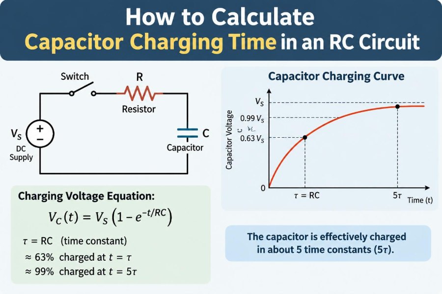
A basic RC circuit contains a resistor, R, and a capacitor, C, connected in series to a DC voltage source. When a switch closes, current flows through the resistor and stores charge on the capacitor.
The resistor limits current. The capacitor develops a voltage that starts at its initial value and rises toward the supply voltage. As capacitor voltage rises, the voltage left across the resistor falls, so charging current steadily decreases.
For the standard charging equation, assume an ideal source with voltage VS, a resistor R, and a capacitor that starts discharged. Real circuits can depart from this model, but it is the correct starting point.
🪣 A Useful Water Analogy
Imagine a water tank being filled through a narrow pipe. The pipe restricts the initial flow, while the rising water level creates pressure that increasingly opposes additional flow.
At first, the tank fills quickly because the difference in pressure is large. As the tank approaches the supply level, filling slows. It gets closer and closer to full but, in the ideal mathematical model, never reaches exactly 100% in a finite time.
The resistor is like the narrow pipe, and the capacitor is like the tank. This analogy explains why capacitor charging is curved rather than a straight, constant-rate ramp.
📈 Why Capacitor Voltage Rises Exponentially
At the instant power is applied to a discharged capacitor, its voltage is 0 V. It behaves momentarily like a short circuit, so the initial current is limited mainly by the resistor: I(0) = VS/R.
As charge accumulates, capacitor voltage VC rises. The resistor voltage becomes VS − VC, and therefore its current becomes smaller. Because capacitor current is proportional to the rate of voltage change, a lower current means a slower rise.
This feedback between voltage and current produces an exponential charging curve. The curve is fast at the beginning and gradually flattens near its final value.
⏱️ Define the RC Time Constant
The central quantity is the time constant, written as the Greek letter tau: τ. It is calculated as:
τ = R × CUse resistance in ohms and capacitance in farads to obtain seconds. For example, 10 kΩ and 100 µF give:
τ = 10,000 Ω × 0.000100 F = 1 secondA time constant does not mean the capacitor is fully charged after one second. It marks a specific, repeatable point on the exponential curve.
🎯 What One Time Constant Means
For a capacitor initially at 0 V and charging toward a DC supply, after one time constant it reaches approximately 63.2% of its final voltage. This value comes directly from the exponential equation.
After two time constants, the capacitor reaches about 86.5%. Each additional time constant removes about 63.2% of the remaining gap between capacitor voltage and final voltage.
This distinction matters. The capacitor does not add another fixed 63.2% each second; instead, it closes a fixed fraction of whatever voltage difference remains.
🧮 The Capacitor Charging Equation
For a capacitor that begins discharged and charges from an ideal DC source, the voltage across it is:
V_C(t) = V_S × (1 − e^(−t/RC))Here, VC(t) is capacitor voltage at time t, VS is supply voltage, e is the base of natural logarithms, R is resistance, and C is capacitance.
The equation shows an important property: the supply voltage sets the final level, while R and C set the curve’s time scale. Doubling the supply voltage does not double the time constant.
🔍 Solving the Equation for Charging Time
Usually, the design question is reversed: “How long until the capacitor reaches a target voltage?” Rearranging the charging equation gives:
t = −RC × ln(1 − V_C/V_S)The term ln is the natural logarithm. The ratio VC/VS must be less than 1 for ordinary charging toward the supply rail.
This equation is more accurate than applying a general “five tau” rule when a circuit responds at a known threshold, such as 2.0 V on a 5 V supply.
📊 Common Charging Percentages and Times
The table below provides convenient reference points for a capacitor starting at 0 V. Multiply the listed number of time constants by RC to calculate time.
| Capacitor voltage as a percentage of final value | Time in time constants | Typical use |
|---|---|---|
| 50% | 0.693τ | Midpoint or threshold calculations |
| 63.2% | 1τ | Definition of one time constant |
| 90% | 2.303τ | Approximate settling target |
| 95% | 2.996τ | Many practical timing applications |
| 99% | 4.605τ | Near-final voltage |
| 99.3% | 5τ | Common “effectively charged” rule |
These values are based on the ideal exponential model. They are excellent for preliminary calculations and often adequate for practical circuits when component tolerances are considered.
🧾 Unit Conversions That Prevent Errors
Most charging-time mistakes are not conceptual; they are unit mistakes. Prefixes must be converted before multiplying R and C.
- 1 kΩ = 1,000 Ω
- 1 MΩ = 1,000,000 Ω
- 1 µF = 0.000001 F
- 1 nF = 0.000000001 F
- 1 ms = 0.001 s
A particularly common error is treating microfarads as farads. A 100 µF capacitor is 100 × 10−6 F, not 100 F. That single error changes a result by one million.
🧪 Worked Example: Reaching a Voltage Threshold
Suppose a 5 V source charges a 10 µF capacitor through a 100 kΩ resistor. The time constant is:
τ = 100,000 Ω × 10 × 10^−6 F = 1 sAssume a circuit must wait until the capacitor reaches 3 V. The required fraction of the supply is 3/5 = 0.6. Substitute into the rearranged equation:
t = −1 s × ln(1 − 0.6)
t = −ln(0.4) s ≈ 0.916 s
So the capacitor reaches 3 V in about 0.92 seconds. Saying “one time constant” would be a useful estimate, but the threshold calculation gives the actual ideal-model result.
🔋 Worked Example: The Five-Time-Constant Rule
Consider a 1 kΩ resistor and a 470 µF capacitor used to soften a voltage change. The time constant is:
τ = 1,000 Ω × 470 × 10^−6 F = 0.47 sAfter five time constants, the elapsed time is 2.35 s. By then, the capacitor is approximately 99.3% of its final voltage.
This does not mean 2.35 s is universally the “charging time.” If the next stage accepts 90% of the final voltage, it responds much sooner, at about 2.303 × 0.47 s, or 1.08 s.
🚫 Why a Capacitor Never Reaches Exactly 100%
The exponential curve approaches the supply voltage asymptotically. That means it gets arbitrarily close without reaching the exact final value at any finite calculated time.
In engineering, “charged” must therefore be defined by a tolerance or a functional threshold. A circuit may consider 95%, 99%, or a particular comparator input voltage to be sufficient.
Physical circuits also have leakage, noise, finite source resistance, and measurement limits. Exact mathematical completion is not a useful design target.
🧭 Choose the Right Definition of ‘Charged’
Before calculating anything, identify what the circuit needs. A visual fade, a timer, a power rail, and a digital reset input can each require a different endpoint.
- Timing delay: calculate to the comparator, transistor, or logic threshold.
- Power-supply settling: specify an acceptable voltage error or ripple limit.
- Analog measurement: use the required accuracy, often expressed as a fraction of final value.
- Human-visible effect: test the perceived result, because human brightness perception is not linear.
A technically correct RC calculation can still be the wrong design calculation if the target voltage was chosen arbitrarily.
🔌 Initial Capacitor Voltage Changes the Result
Not every capacitor starts discharged. In a repeating circuit, a timing capacitor may retain charge between cycles, or a capacitor may begin at a known precharge voltage.
For a capacitor starting at V0 and charging toward VS, use:
V_C(t) = V_S + (V_0 − V_S) × e^(−t/RC)To find time for a target voltage VT, rearrange it as:
t = −RC × ln((V_T − V_S)/(V_0 − V_S))Check that the target lies between the initial and final voltages. Otherwise, the requested transition cannot occur under those conditions.
🔄 Charging and Discharging Use Related Curves
When a charged capacitor discharges through a resistor toward 0 V, its voltage follows:
V_C(t) = V_0 × e^(−t/RC)The same time constant applies if the discharge path has the same resistor. After one τ, the voltage has fallen to 36.8% of its starting value; after five τ, it is about 0.67%.
Do not automatically assume charging and discharging times match. A diode, transistor, switch resistance, or separate resistor can create different paths and therefore different time constants.
🧱 Source Resistance Becomes Part of R
The simple equation assumes the source has zero internal resistance. A battery, signal generator, microcontroller pin, or power supply actually has some output resistance or current limit.
Resistance in series with the capacitor’s charging path contributes to the effective R. If a 10 kΩ timing resistor is driven by a source with 100 Ω output resistance, the ideal estimate uses approximately 10.1 kΩ.
For a large external timing resistor, this difference may be negligible. For low-resistance, high-current charging, source impedance can dominate the behavior and should not be ignored.
🧩 Capacitor ESR and Leakage Affect Real Timing
Real capacitors have equivalent series resistance, called ESR, and finite insulation resistance, represented by leakage current. ESR causes an immediate voltage drop under changing current, while leakage can prevent a capacitor from reaching the expected voltage in high-resistance circuits.
Leakage matters especially with large electrolytic capacitors, long delays, high temperatures, and megohm-range resistors. In such cases, the charging current late in the cycle can become comparable to leakage current.
For precise or long-duration timers, consult the capacitor data sheet and evaluate leakage at the intended voltage and temperature. A lower-leakage film capacitor or a different timing approach may be more suitable.
🌡️ Component Tolerance and Temperature Drift
A calculated value is only as exact as the components. Resistors are often available with relatively tight tolerances, but many common capacitors have much wider capacitance tolerance.
Because τ = RC, percentage errors approximately add in the worst-case direction. For example, a resistor that is high by its tolerance and a capacitor that is also high produce a longer delay than the nominal calculation.
Temperature can shift capacitance, leakage, and resistance. If a delay must remain accurate across environmental conditions, calculate a tolerance range rather than relying on a single nominal time.
📐 Calculate Best-Case and Worst-Case Delay
For a threshold-based delay, calculate the shortest and longest plausible time using the extreme R and C values. Keep the voltage threshold assumptions consistent with the rest of the circuit.
As a simple first approximation:
τ_min = R_min × C_min
τ_max = R_max × C_max
Then apply the same threshold multiplier, such as 0.693 for 50% or 2.303 for 90%. If the threshold itself varies—as it often does with transistor or logic inputs—include that variation too.
This approach turns an attractive nominal delay into a design you can assess for reliability.
💡 Logic Inputs and Threshold Uncertainty
An RC network connected directly to a digital input can be convenient, but it deserves caution. A standard logic input may have a threshold range rather than one guaranteed switching voltage.
That range translates directly into timing uncertainty. Noise or a slowly changing input can also cause multiple transitions or extra current in some logic families.
A Schmitt-trigger input is often a better choice for an RC-generated signal. Its hysteresis provides separate rising and falling thresholds, improving noise immunity, though the exact threshold values must still be checked for timing accuracy.
🛎️ Comparators Make RC Timing More Predictable
A comparator compares capacitor voltage with a known reference voltage. The output changes state when the two voltages cross, making the intended timing condition explicit.
Compared with relying on an undefined transistor turn-on point or a broad logic threshold, a comparator can provide a more controlled result. Adding hysteresis can prevent noise from causing output chatter near the switching point.
The reference voltage must itself be stable enough for the required accuracy. If the reference tracks the same supply that charges the capacitor, some supply-voltage changes may cancel; if it is independent, they may not.
🧠 When Supply Voltage Does and Does Not Matter
If both the capacitor charging voltage and the switching threshold are fixed fractions of the same supply, the ideal time is independent of supply magnitude. For example, reaching 50% of VS always takes 0.693RC.
If the threshold is an absolute voltage, supply voltage matters. A 2 V threshold is 40% of a 5 V supply but only about 16.7% of a 12 V supply, so the time to reach it changes substantially.
This distinction is useful when designing battery-powered equipment, where the supply changes as the battery discharges.
🔧 Selecting R and C Values for a Desired Delay
Start from the required threshold multiplier, then solve for the needed time constant. If a capacitor must reach 90% in 1 s, τ must be approximately 1/2.303, or 0.434 s.
Next choose practical component values whose product is close to that value. A 47 kΩ resistor and a 10 µF capacitor give 0.47 s, which is a reasonable nominal starting point.
There is rarely one perfect pair. Choose values while considering capacitor type, leakage, resistor power, available package sizes, adjustment needs, and the impact of tolerances.
⚠️ Avoid Extremely Large Resistances Without Checking Leakage
A 10 MΩ resistor appears attractive for creating long delays with a small capacitor. However, charging current can then be very small, making capacitor leakage, board contamination, humidity, and input bias current significant.
For example, a few hundred nanoamps of unwanted current can materially affect a node intended to charge through megohms. The ideal RC equation no longer describes the circuit well unless those currents are modeled.
For long, accurate delays, consider a low-leakage capacitor, a buffered node, a comparator with low input bias current, or a digital timer and clock source.
🔥 Avoid Very Small Resistances With Large Capacitors
At the other extreme, a large capacitor connected through a very small resistance draws a high inrush current at turn-on. The ideal initial current is VS/R, but a real source may current-limit or sag.
The resistor, switch, regulator, connector, and capacitor ESR must tolerate the pulse. A resistor chosen only for its time constant may dissipate substantial short-term power during charging.
Use the resistor’s pulse rating where relevant, and remember that a bench supply’s current limit can dramatically alter the observed waveform.
📟 Measure Charging Time With an Oscilloscope
An oscilloscope shows the exponential waveform directly. Connect the probe ground to circuit ground and measure the capacitor node, using a probe setting and input impedance appropriate for the circuit.
Trigger on the switching event, then use cursors to measure the time from the start of charging to the target voltage. Compare that result with the theoretical value and expected tolerance range.
Be careful: a probe adds capacitance and resistance. In a low-impedance circuit this is usually insignificant, but it can alter timing noticeably with very small capacitors or very high-value resistors.
🧰 Measure With a Multimeter When a Scope Is Unavailable
A digital multimeter can confirm the general rise of capacitor voltage, but it is poorly suited to fast transitions and may update too slowly to capture a timing point accurately.
For slow RC circuits, record the capacitor voltage at known intervals or use a meter with logging capability. Ensure that the meter’s input impedance is much higher than the resistor in the timing network.
If a 10 MΩ-input meter measures a node charged through several megohms, the meter becomes a parallel resistance and can change the result. Measurement equipment is part of the circuit while connected.
❌ Common Calculation Mistakes
Several errors appear repeatedly in RC timing work:
- Calling one time constant the full charging time.
- Using 5τ when the circuit actually responds at a lower threshold.
- Mixing microfarads, nanofarads, milliseconds, and base SI units.
- Ignoring initial capacitor voltage in repetitive operation.
- Assuming the source, input, and capacitor are ideal.
- Using a nominal calculation without checking tolerances.
- Forgetting that a meter or oscilloscope probe can load the node.
Most of these issues are easy to avoid by drawing the actual current path, defining the trigger voltage, and checking which nonideal elements are large enough to matter.
🧷 A Practical Calculation Workflow
A disciplined workflow makes RC calculations quick and defensible:
- Identify the initial capacitor voltage, final voltage, and target voltage.
- Find the total effective resistance in the charging path.
- Convert all units to ohms, farads, and seconds.
- Calculate τ = RC.
- Use the threshold equation, or a known time-constant multiplier.
- Evaluate resistor and capacitor tolerances, leakage, source resistance, and threshold uncertainty.
- Verify the result on the actual circuit, especially when timing is critical.
This process works equally well for a simple classroom calculation and a more careful design review.
🧑🏭 Where RC Charging Calculations Are Used
RC charging appears in delay-on circuits, power-on reset networks, debounce filters, analog smoothing, pulse stretching, ramp generation, sensor conditioning, and soft-start functions.
In a debounce circuit, the goal is often to reject short switch disturbances rather than create an exact delay. In a power-on reset circuit, the relevant issue may be whether a threshold is crossed cleanly during a supply ramp.
The same equation applies, but the engineering requirement changes. Understanding the surrounding circuit is what turns a formula into a useful design decision.
✅ The Core Principle to Remember
Capacitor charging time is governed by an exponential relationship, not a constant-rate rise. The product RC sets the time scale, and the required fraction of the final voltage determines how many time constants are needed.
For a discharged capacitor charging toward VS, use t = −RC ln(1 − VC/VS) whenever you know the target voltage. Use the five-time-constant approximation only when “near the final value” is genuinely sufficient.
Finally, treat ideal calculations as a baseline. Source resistance, capacitor leakage, tolerances, thresholds, temperature, and measurement loading decide whether the physical circuit matches the number on paper.
Calculate the required voltage threshold first, then use the RC time constant to find the delay that your real circuit—not just an ideal diagram—will produce. 🔌⏱️🧪