
A robot arm stops at a commanded angle without shaking. A 3D printer holds its nozzle near the selected temperature. An electric motor reaches a target speed even when its load changes. These everyday results depend on feedback control.
Without feedback, an actuator only follows an instruction: apply a voltage, open a valve, or deliver heater power. Real systems are less cooperative. Loads vary, friction changes, heat escapes, sensors contain noise, and delays make a simple command inaccurate.
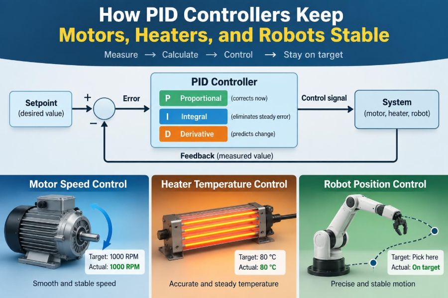
A PID controller continuously compares what a system should do with what it is actually doing. It turns the difference into a corrective action using proportional, integral, and derivative terms.
PID control is one of the most useful ideas in electronics engineering because the same structure can regulate speed, position, temperature, pressure, flow, and many other physical quantities. Understanding it means learning how embedded hardware makes dynamic systems behave predictably. ⚙️
🎯 1. The control problem in one question
Every closed-loop controller addresses a simple question: how should the input change so that the measured output reaches the desired value? The desired value is the setpoint, also called the reference.
For a motor-speed loop, the setpoint may be 1,500 rpm. For a heater, it may be 200 °C. For a mobile robot, it might be a wheel speed, heading, or distance from a wall.
The controller does not directly know the ideal input in advance. Instead, it keeps correcting its command as new sensor measurements arrive.
🔄 2. Open loop versus closed loop
An open-loop system sends a command but does not check the result. A heater driven at a fixed duty cycle is open loop if its temperature is never measured.
A closed-loop system measures the output and feeds that information back to the controller. If the room gets colder, a temperature controller can raise heater power; if a motor is loaded, a speed controller can increase drive effort.
| Feature | Open-loop control | Closed-loop control |
|---|---|---|
| Measurement of output | Not used for correction | Continuously or periodically used |
| Response to disturbances | Usually cannot compensate | Can reject many disturbances |
| Design complexity | Lower | Higher because sensing and tuning are needed |
| Typical example | Fixed PWM motor drive | Encoder-based speed control |
📏 3. Error is the signal that drives action
The controller begins with the error, commonly written as e(t). It is the reference minus the measured process variable:
e(t) = r(t) - y(t)Here, r(t) is the setpoint and y(t) is the measured output. A positive error means the output is below the requested value when this sign convention is used.
Correct sign matters. If positive error makes the actuator push the output farther away from the setpoint, the loop has positive feedback and may run away instead of stabilizing.
🧩 4. What PID means
PID stands for proportional, integral, and derivative. The classical continuous-time equation is:
u(t) = Kp e(t) + Ki ∫e(t)dt + Kd de(t)/dtu(t) is the controller output, such as a PWM duty cycle, valve command, current reference, or heater-power command. The gains Kp, Ki, and Kd determine how strongly each term contributes.
The equation is compact, but each term addresses a different weakness of a physical system. Good PID design is mostly the practical art of balancing those contributions.
📈 5. Proportional action: respond to the present
The proportional term is Kp e(t). It creates an output directly proportional to the current error, so a large error produces a stronger correction.
Increasing Kp often makes a loop react faster and reduces error during a change in setpoint. In a motor, it can raise drive voltage quickly when speed falls below the target.
Too little proportional gain gives a slow, weak response. Too much can produce overshoot, oscillation, excessive current demand, or audible motor noise. Proportional action alone often leaves a remaining offset under constant load.
🧮 6. Integral action: remember the past
The integral term accumulates error over time. Even a small persistent error keeps adding to the integral state, gradually increasing the correction until the mismatch is removed.
This is why integral action eliminates steady-state error in many applications. A speed controller with integral gain can supply the extra motor torque needed to overcome a constant load rather than settling permanently below the requested speed.
Integral action is powerful but patient. It can also become harmful when the actuator reaches a limit and the integral state continues accumulating error.
⚡ 7. Derivative action: react to the trend
The derivative term responds to how quickly the error changes. It acts like a prediction based on the current trend: if the output is racing toward the setpoint, derivative action can reduce the command before a large overshoot develops.
Appropriate Kd can add damping to a lightly damped mechanical system, such as a position-controlled motor or robot joint. It is often helpful where inertia and resonance make the response bouncy.
A derivative is sensitive to rapid measurement changes, including sensor noise. For this reason, practical derivative implementations almost always use filtering and are sometimes omitted entirely.
🪣 8. Build intuition with a water tank
Imagine controlling water level in a tank by adjusting an inlet valve. If the level is below target, proportional action opens the valve according to the size of the gap.
If a small gap remains because outflow is constant, integral action slowly opens the valve further until inflow matches outflow. If the water level rises rapidly toward the target, derivative action can begin closing the valve sooner.
The tank makes two important facts visible: physical systems store energy or material, and they respond over time rather than instantly. Motors and thermal systems have the same dynamic character.
🌡️ 9. Why heaters are a classic PID application
A heater has thermal mass, heat loss to its surroundings, and a delayed sensor response. Applying full power does not make the sensor temperature jump immediately; the temperature rises gradually, often continuing upward after power is reduced.
A PID loop measures temperature and adjusts power, usually through time-proportioned switching, PWM, or a power-control stage. Proportional action supplies immediate correction, while integral action compensates for steady heat loss.
Derivative action may help in some thermal plants, but noisy sensors and slow sampling can make it less useful than careful PI control. Many temperature loops work well with only proportional and integral terms.
🛞 10. Speed control for DC and BLDC motors
A motor’s speed depends on applied voltage or current, supply voltage, back EMF, friction, and load torque. A fixed PWM duty cycle therefore does not guarantee a fixed speed.
With an encoder, Hall sensors, or an observer, the controller estimates speed and compares it with the target. The PID output may set PWM duty cycle directly, but in higher-performance drives it often becomes a torque or current reference.
When a conveyor receives a heavier item, its motor slows briefly. A well-tuned speed loop detects the error and increases drive effort, restoring speed without a large visible sag.
🦾 11. Position control needs a layered view
A position loop commands where a shaft or joint should be, using a potentiometer, encoder, or resolver as feedback. The controller must manage inertia, friction, gearbox backlash, and the fact that motor torque creates acceleration before it creates position change.
Many servo systems use cascaded loops. An outer position loop generates a speed command, a middle speed loop generates a torque or current command, and a fast inner current loop regulates motor current.
Each inner loop is normally faster than the loop around it. This separation makes the overall system easier to tune and gives fast protection against torque disturbances.
🤖 12. Robots use feedback everywhere
A mobile robot may run separate PID loops for left and right wheel speed. Equal commands alone do not ensure a straight path because wheel friction, motor constants, and battery voltage differ.
A balancing robot uses inertial sensors to estimate tilt and applies motor torque to oppose falling. A robot arm regulates joint position, often with extra compensation for gravity, friction, and changing load.
Common robot control loops
- Wheel-speed regulation for accurate motion.
- Heading control using encoder, gyro, or fused estimates.
- Joint position and velocity regulation.
- Temperature control for batteries, motors, or processing hardware.
PID is not the entire robotics stack, but it is often the dependable low-level layer that turns planning decisions into stable motion.
⏱️ 13. Sampling turns a physical controller into code
Microcontrollers execute PID at discrete intervals, not continuously. At each sample, firmware reads a sensor, calculates the control output, limits it if necessary, and updates the actuator.
The sample period, often written dt, is part of the design. A loop sampled too slowly cannot observe or correct rapid changes well; a loop sampled much faster than necessary may waste processor time and expose more sensor noise.
Timing should be consistent. A timer interrupt or real-time scheduling mechanism is usually preferable to running the controller whenever the main loop happens to reach it.
💻 14. A practical discrete PID equation
A common discrete implementation updates an integral state and estimates a derivative from differences between samples:
error = setpoint - measurement
integral = integral + error * dt
derivative = (error - previous_error) / dt
output = Kp * error + Ki * integral + Kd * derivative
previous_error = error
The output then passes through saturation limits appropriate for the hardware, such as 0 to 100% duty cycle or a signed command range. Units must stay consistent: seconds for dt, meaningful sensor units for error, and known actuator units for output.
This simple form is useful for learning, but production firmware needs protections for noise, limits, mode changes, and invalid sensor data.
🧱 15. Actuator saturation changes the problem
No physical actuator has unlimited authority. A heater cannot deliver more than its rated power, and a battery-powered motor driver cannot command voltage beyond the supply rail.
When the output reaches a maximum or minimum, the plant cannot respond with the correction that the PID equation requests. Large errors can remain even though the software keeps asking for more.
Designers should explicitly clamp the command and consider the consequences. Saturation is not merely a software detail; it strongly affects transient behavior and integral action.
🌪️ 16. Integral windup and anti-windup
Integral windup occurs when the integral term accumulates while the output is saturated. For example, a cold heater may stay at full power for a long time, building a large integral state before the temperature nears its target.
Once the process can respond, that stored integral command can cause severe overshoot and a slow recovery. The same issue appears when a motor is blocked or a robot hits a mechanical stop.
Useful anti-windup approaches
- Stop integrating when the output is saturated and the error would push it further into saturation.
- Clamp the integral state to a selected range.
- Use back-calculation to drive the integral state toward the achievable output.
- Reset or preload the integrator carefully during operating-mode changes.
📡 17. Sensors define what the controller can know
A controller only sees the measured value, not the true physical state directly. Sensor resolution, offset, calibration, latency, quantization, and mounting all affect the feedback signal.
An encoder with limited counts per revolution produces a speed estimate that can be coarse at low speed. A thermistor may be accurate at its location but respond slowly to the temperature of the object that actually matters.
Before blaming PID gains, verify the sensor path. Check scaling, sign, filtering, update rate, electrical noise, and whether the sensor is measuring the intended variable.
📉 18. Noise, derivative, and filtering
Differentiation amplifies high-frequency content. Since measurement noise often changes rapidly, calculating derivative directly from a noisy error can produce a jittery actuator command.
One common alternative is derivative on the measurement rather than on the error. This avoids a large derivative kick when the setpoint changes suddenly, because the measured output does not jump at the same instant.
A low-pass filter on the derivative estimate can help, but filtering also adds delay. The aim is not to erase every fluctuation; it is to suppress noise without removing useful dynamic information.
🚦 19. Setpoint changes deserve careful handling
A step setpoint asks the system to change immediately, which may demand unrealistic torque, current, or heater power. In a robot, abrupt commands can excite resonances or cause wheel slip.
Setpoint ramping limits how quickly the reference changes. Trajectory generators can also limit acceleration and jerk, producing commands that are easier for the plant and PID loop to follow.
For many systems, a smoother command improves results more effectively than increasing gains. The controller should regulate a physically achievable target, not fight an impossible demand.
📊 20. Reading the step response
A step test changes the setpoint and records the response. It provides a practical picture of speed, damping, accuracy, and stability.
Terms to recognize
- Rise time: how quickly the output approaches the new target.
- Overshoot: how far the response exceeds the target.
- Settling time: how long the response takes to remain near target.
- Steady-state error: the remaining difference after transients fade.
- Oscillation: repeated motion around the target, often caused by inadequate damping or excessive gain.
No single metric is always best. A precision position stage may prioritize low overshoot, while a motor-speed loop may accept modest overshoot to reject load disturbances quickly.
🎛️ 21. Start tuning with a safe test setup
Tuning is an experiment on a real dynamic system, so start with safety limits. Secure moving hardware, limit travel, set conservative current limits, ensure cooling, and log the setpoint, measurement, and output.
Begin with a known controller direction and small gains. Confirm that a positive control effort moves the measured variable in the expected direction before attempting aggressive tests.
Make one meaningful change at a time. A record of gains, load conditions, supply voltage, sampling period, and response plots prevents tuning from becoming guesswork.
🧭 22. A practical manual tuning sequence
A common starting method is to set integral and derivative gains to zero, then increase proportional gain until the response is adequately fast but not excessively oscillatory. The acceptable point depends on the plant and its safety margins.
Next, add integral gain gradually to remove persistent offset. Watch for slow oscillation or overshoot, which may indicate too much integral action or actuator saturation.
Add derivative only if extra damping is needed and the measurement supports it. Then retest with realistic disturbances, operating ranges, and setpoint changes rather than judging performance from one ideal test.
🧪 23. Test disturbances, not just commands
Following a setpoint is only half the job. A useful control loop also rejects disturbances: a changed load torque, a supply variation, a draft around a heater, or a robot moving over a different floor surface.
For a speed loop, apply a safe load change and observe the speed dip and recovery. For a thermal loop, observe behavior when ambient conditions or heat loss changes.
A system that looks excellent in an unloaded bench test may behave poorly in operation. Tune and validate under the conditions that matter to the product.
🧰 24. Feedforward complements feedback
Feedback reacts after an error appears. Feedforward uses known information to command an expected input before a significant error develops.
A motor controller can add a voltage or torque estimate based on desired speed and acceleration. A robot arm can add a gravity-compensation torque based on joint angle. A heater can include an estimated baseline power for normal heat loss.
Feedforward does not replace PID because models are imperfect and disturbances remain. It reduces the burden on feedback, allowing smaller errors and less aggressive gains.
🔗 25. When PI, PD, or P control is enough
Not every loop needs all three terms. The right controller structure follows from plant behavior, sensor quality, performance needs, and safety constraints.
- P control can be suitable where some steady error is acceptable and simplicity matters.
- PI control is common for speed, current, flow, and temperature loops because it removes steady offset without requiring noisy differentiation.
- PD control can add damping where offset is handled elsewhere or naturally unimportant.
- PID control is useful when proportional response, zero steady error, and added damping are all needed.
Adding a term simply because the letters are available is not good engineering. Each term should solve an observed problem.
🛡️ 26. Reliability and safety belong around the PID loop
A PID algorithm should not be the only protection in a system. Independent hardware and firmware safeguards are needed because sensors, actuators, wiring, and software can fail.
Examples include overcurrent protection, thermal cutoffs, watchdog timers, travel limit switches, plausibility checks, output-rate limits, emergency stop behavior, and a defined safe state after sensor loss.
Also consider startup and shutdown. Initializing the integrator to zero may create a command jump; preserving or preloading a suitable state can make transitions smoother when it is safe to do so.
🧠 27. The core principle: correct, observe, repeat
A PID controller keeps a system stable by repeating a disciplined cycle: measure the output, compare it with the target, calculate a correction, apply the correction, and measure again. Proportional action addresses the present error, integral action addresses accumulated error, and derivative action addresses the changing trend.
Stable results come from more than three gains. They require correct feedback direction, appropriate sampling, trustworthy sensors, realistic commands, actuator limits, anti-windup, and testing against real disturbances.
PID control succeeds when the controller, sensor, actuator, and physical plant are designed as one feedback system—not as isolated parts. ⚙️ 🤖 📈