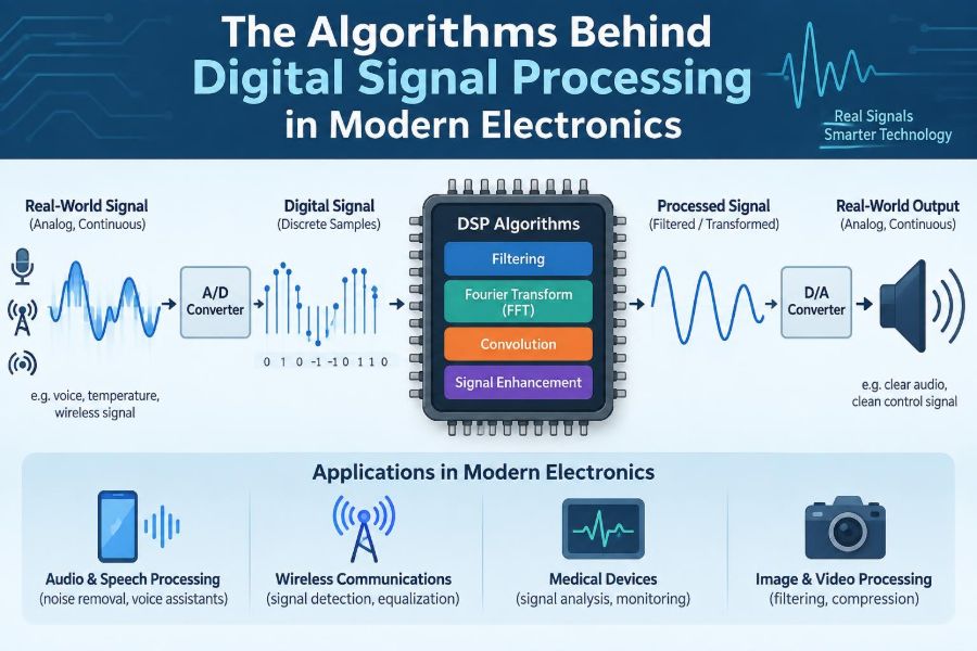

Your wireless earbuds suppress a train’s rumble while preserving a podcast voice. Your phone turns a faint radio signal into a clear call. A smartwatch separates a heartbeat from motion caused by walking. None of these devices works by simply “reading” electricity.
They measure changing voltages, represent those measurements as numbers, and repeatedly transform those numbers using carefully chosen algorithms. This is digital signal processing, usually shortened to DSP.
DSP is one of the quiet foundations of modern electronics. It appears in audio equipment, cameras, medical instruments, motor drives, radar, power converters, industrial sensors, and communications hardware.
The useful question is not only what an algorithm does, but why its assumptions fit a real signal, a physical sensor, and a limited processor. That connection between mathematics and hardware is where good electronics engineering happens.
📡 A Signal Is Information Carried by Change
A signal is a measurable quantity that varies in a way that conveys information. Voltage from a microphone, light reaching an image sensor, acceleration from an inertial sensor, and current in a power system can all be signals.
Some signals are continuous in time and amplitude. Others are represented as sequences of discrete numbers. DSP focuses on processing the numerical sequence while keeping its relationship to the original physical quantity meaningful.
🔄 Why Digital Processing Replaced Many Analog Functions
Analog circuits can filter, amplify, mix, and detect signals directly. They remain valuable, particularly at very high frequencies, in low-power front ends, and where extremely low latency is required.
Digital processing adds flexibility. A filter’s behavior can be changed in firmware, duplicated accurately across products, adapted to changing conditions, or combined with decisions such as classification and control.
The trade-off is that a digital system needs conversion, computation, memory, clocking, and power. DSP does not eliminate analog design; it makes a carefully designed analog-digital chain possible.
🎛️ The Signal Chain Starts Before the Algorithm
A typical chain begins with a sensor and an analog front end. The front end may amplify a tiny signal, reject unwanted common-mode interference, shift its level, and limit its bandwidth before conversion.
An analog-to-digital converter, or ADC, produces samples. A processor, FPGA, DSP chip, or microcontroller runs algorithms on them. If the result must drive a speaker, actuator, or analog control input, a digital-to-analog converter and output conditioning follow.
A weak front end cannot usually be repaired by sophisticated code. Clipping, inadequate sensor resolution, and severe interference can destroy information before a DSP routine sees it.
🧮 Sampling Turns Time Into a Sequence
Sampling measures a signal at regular time intervals. If samples are taken every T seconds, the sampling frequency is 1/T samples per second. A sequence may be written as x[n], where n identifies the sample number.
A waveform that changes slowly relative to the sample rate is represented by many points. A waveform near the sampling limit has few points per cycle, making its timing and shape harder to interpret accurately.
Regular sampling simplifies algorithm design because the processor can treat time as an ordered index. In practice, the sampling clock’s stability also matters; clock variation can become distortion or timing error.
⚠️ Nyquist Explains the Need for Bandwidth Control
For a band-limited signal, the familiar sampling condition is that the sample rate must exceed twice the highest frequency of interest. This is often called the Nyquist criterion.
It is not a license to sample only barely above the limit. Real filters need a transition band: a region where unwanted frequencies are being attenuated rather than removed instantly. Engineers commonly choose extra margin so the analog filter is practical.
For example, a sensor channel intended to preserve content below a certain band edge must attenuate higher-frequency energy before sampling. Otherwise, that energy can enter the stored sequence under a false identity.
🪞 Aliasing Folds Frequencies Into the Wrong Place
Aliasing occurs when different continuous-time frequencies produce indistinguishable sampled sequences. A frequency above half the sample rate can appear as a lower frequency after sampling.
This is not merely a cosmetic problem. In vibration monitoring, an aliased component can be mistaken for a real machine fault frequency. In audio, it can create inharmonic tones. In control systems, it can corrupt the feedback measurement.
The principal defense is an anti-aliasing low-pass filter before the ADC. Increasing the sample rate can help, but it does not remove the need to consider frequencies, noise, and interference above the intended band.
🔢 Quantization Gives Samples Finite Precision
An ADC must map a continuous voltage range to a finite set of codes. This mapping is quantization. With more bits, the spacing between available codes becomes smaller for a fixed input range.
Quantization creates error because most input values lie between codes. For many signals and operating conditions, that error behaves somewhat like added noise, but it can also show patterns when the signal is very small or highly repetitive.
Resolution alone is not performance. Noise in the reference, ADC nonlinearity, incorrect input range, and poor grounding can prevent a converter from achieving the useful precision suggested by its nominal bit count.
📏 Dynamic Range Sets What Can Be Seen
Dynamic range describes the span between the largest usable signal and the smallest signal that can be distinguished from noise or error. A recording device must accommodate loud peaks without clipping while still resolving quiet detail.
Gain selection is therefore an engineering decision, not a simple “maximize amplitude” rule. Too little gain wastes converter range; too much causes clipping, which introduces broadband distortion that later filtering cannot truly undo.
Automatic gain control can adapt levels, but its time constants must fit the application. Fast adjustment may protect against overload, while unwanted gain motion can make a measurement or audio recording misleading.
➕ Convolution Is the Core Operation of Many DSP Systems
Convolution combines an input sequence with a second sequence called an impulse response. It expresses the idea that each input sample causes a response extending over time, and all those responses add together.
For a finite impulse response filter, the calculation is a weighted sum of recent samples:
y[n] = b[0]x[n] + b[1]x[n-1] + ... + b[M]x[n-M]The coefficients b determine what the filter does. By choosing them carefully, a designer can smooth noise, isolate a band, compensate a sensor, or shape an audio response.
🧹 FIR Filters Offer Predictable Behavior
A finite impulse response, or FIR, filter uses a finite number of past input samples. Its output depends on the input history but not on previous outputs.
FIR filters are valued because they can be designed with exact linear phase. Linear phase means frequency components are delayed by the same amount, preserving waveform shape apart from delay. This can matter in data acquisition, audio processing, and multichannel measurement.
The cost is computation: narrow transitions or strong stop-band attenuation may require many coefficients. Efficient implementation and suitable hardware become important at high sample rates.
🔁 IIR Filters Achieve Sharp Responses Efficiently
An infinite impulse response, or IIR, filter feeds previous output values back into its calculation. This feedback allows a sharp frequency response with relatively few coefficients.
Classic analog filter families can be translated into digital IIR structures, which is one reason they are common in embedded systems. A biquad, a second-order IIR section, is a widely used building block.
Feedback also creates risk. Coefficient rounding, overflow, and an unsuitable structure can make a theoretically stable filter behave poorly or even become unstable in fixed-point hardware.
⚖️ Choosing Between FIR and IIR
| Consideration | FIR approach | IIR approach |
|---|---|---|
| Phase behavior | Can provide exact linear phase | Usually nonlinear phase |
| Computation for sharp filters | Often higher | Often lower |
| Stability | Inherently stable with finite coefficients | Must be checked carefully |
| Common fit | Resampling, data paths, waveform preservation | Low-cost embedded filtering, control conditioning |
Neither filter type is universally better. The correct choice depends on phase requirements, latency, available memory, processor load, coefficient precision, and the required attenuation.
🪟 Windows Manage Finite Measurements
Algorithms often analyze a short block of samples rather than an endless sequence. Cutting out a block is equivalent to multiplying the signal by a rectangular window, which can cause spectral leakage when the block does not contain an exact whole number of cycles.
A tapered window reduces the sharp discontinuity at the block edges. Different windows balance main-lobe width, which affects frequency separation, against side-lobe level, which affects leakage from strong nearby tones.
Window selection should follow the measurement goal. A window that reveals a small tone near a large one may not give the same frequency resolution as a different choice.
🌈 The FFT Reveals Frequency Content Efficiently
The discrete Fourier transform describes a block of samples as a set of frequency components. The fast Fourier transform, or FFT, is an efficient algorithm for calculating that transform.
An FFT does not create extra information; it reorganizes the available information into frequency bins. The spacing between bins depends on sample rate and transform length. Longer records provide closer bin spacing but increase delay and may be less suitable for rapidly changing signals.
A spectrum analyzer, a music visualizer, and many diagnostic tools use FFT-based processing. Interpreting their display correctly requires attention to windowing, scaling, averaging, and whether the input is stationary during the measurement.
🎵 Spectrograms Show Change Over Time
A single FFT gives a frequency snapshot for one block. A spectrogram calculates overlapping FFTs and displays their magnitude across time and frequency.
This is useful for speech, machine sounds, radar returns, and transient events. The block length creates a time-frequency trade-off: short blocks track rapid changes but blur close frequencies, while long blocks separate frequencies better but smear timing.
That trade-off is a property of the analysis, not a software flaw. Engineers choose settings based on what event they need to distinguish.
🧭 Phase Carries Timing and Alignment Information
Magnitude says how much of a frequency is present. Phase describes its position within a cycle relative to a reference. Ignoring phase can be acceptable for some displays, but it can be disastrous for reconstruction, beamforming, synchronization, and feedback control.
Two equal signals can cancel if they are combined with opposite phase. Conversely, accurate phase alignment lets microphone arrays emphasize sound from one direction or lets communication receivers recover a carrier reference.
Phase can be sensitive to delay. Even one sample of timing mismatch between channels may matter when signals are combined at higher frequencies.
🧭 Complex Numbers Make Modulation Practical
Many communication and radar systems represent signals using in-phase and quadrature components, called I and Q. Together they form a complex-valued sample, with one component treated as real and the other as imaginary.
This representation makes frequency shifts, phase rotation, amplitude estimation, and modulation easier to express. It also distinguishes positive and negative frequency behavior in a useful mathematical way.
In a software-defined radio, for example, I/Q samples can be digitally filtered and shifted to isolate a desired channel without rebuilding the analog radio for every channel plan.
📻 Modulation Moves Information Through Real Channels
Modulation places information onto a carrier by changing amplitude, frequency, phase, or a combination of these. A receiver must estimate timing, carrier frequency, phase, and channel effects before it can reliably recover symbols or audio.
DSP algorithms perform tasks such as matched filtering, symbol timing recovery, equalization, and error detection. Their settings depend on the modulation method and on impairments such as noise, multipath reflections, oscillator mismatch, and interference.
Real channels rarely match textbook assumptions exactly. Robust receiver design includes margins and monitoring for cases where synchronization begins to fail.
🧩 Correlation Finds Similarity and Delay
Correlation compares one sequence with a shifted version of another sequence. A strong peak indicates that the patterns align well at a particular delay.
GPS-style ranging concepts, packet detection, sonar, synchronization preambles, and time-delay estimation all rely on correlation. A known reference pattern is searched for inside a received signal.
The reference must be distinctive enough to avoid false peaks, and the search process must account for noise, frequency offset, and multipath. A clean-looking peak is evidence of alignment, not always proof of a unique physical path.
🧠 Adaptive Filters Learn From Their Error
An adaptive filter changes its coefficients while operating. Instead of using a fixed response, it observes an error signal and adjusts toward lower error according to a chosen update rule.
Noise cancellation is a familiar example. If a reference microphone captures a correlated noise source, an adaptive filter can estimate how that noise reaches the main microphone and subtract an estimate.
Adaptation has limits. The reference must be sufficiently correlated with the unwanted signal, and fast changes can require faster adaptation, which may increase sensitivity to noise or interfere with the desired content.
🗜️ Compression Reduces Data, Not Necessarily Quality
Compression reduces the number of bits needed to store or transmit information. Lossless methods preserve every original digital value; lossy methods discard or approximate information judged less relevant for a particular use.
Audio and image compression often exploit statistical redundancy and perceptual limits. The result can be efficient, but repeated encoding or aggressive settings can introduce artifacts such as ringing, blocking, or altered high-frequency detail.
For scientific measurement, legal evidence, calibration records, or future reanalysis, raw or lossless data may be preferable. The right choice follows the purpose of the data, not file size alone.
🧱 Fixed-Point Arithmetic Changes Algorithm Design
Many low-cost and low-power processors use fixed-point arithmetic, where numbers have a predetermined scaling rather than a freely varying floating-point exponent. This can be efficient and predictable, but the numerical range is limited.
Designers must select word lengths, scaling points, rounding behavior, and saturation rules. Overflow that wraps around can produce a large, nonsensical sign change; saturation often fails more gracefully but still distorts the signal.
Testing only with normal inputs is insufficient. A robust design exercises maximum amplitudes, startup transients, coefficient extremes, and combinations of tones that create high internal peaks.
⏱️ Latency Is a System Requirement
Every block buffer, filter, converter, and communication step adds delay. In offline analysis, this may not matter. In hearing assistance, active noise control, motor protection, or closed-loop control, it can determine whether the system works.
Latency is not simply processor execution time. It includes ADC and DAC conversion delay, buffering, scheduler delays, transport delays, and group delay from filters.
Lower latency may require shorter blocks or simpler filters, but those choices can reduce frequency resolution or attenuation. Good designs state the latency budget early rather than treating it as a late optimization.
⚡ Real-Time DSP Requires Deterministic Scheduling
A real-time system must finish each processing task before the next critical data deadline. Average speed is not enough; occasional deadline misses can cause dropped samples, audible glitches, or unsafe control behavior.
Direct memory access, interrupt design, double buffering, and priority assignment are practical tools for moving data reliably. The algorithm must be measured on the target hardware, because cache behavior and peripheral contention can affect timing.
Profiling identifies where cycles go, but worst-case behavior deserves attention too. A routine that is fast most of the time may still fail when an unusual packet, interrupt burst, or branch path occurs.
🔋 Power and Memory Put Boundaries Around the Math
Battery-operated products cannot treat computation as free. More multiplications, higher sample rates, frequent memory access, and radio transfers can all raise energy use.
Memory placement also matters. A filter with many coefficients may be mathematically suitable but impractical if it causes frequent external-memory access or exceeds the available fast memory.
Decimation and multirate processing are useful strategies. A system can filter then reduce the sample rate once high-frequency content is no longer needed, cutting the processing required by later stages.
🧪 Validation Needs Signals That Expose Failure Modes
A DSP chain should be tested with more than a pleasant-looking waveform. Sine sweeps, impulses, steps, multitone signals, noise, clipped inputs, and realistic recorded data expose different properties.
Useful checks include gain, frequency response, phase or group delay, noise floor, overload recovery, stability, and sensitivity to clock or coefficient errors. For communication algorithms, test impaired channels rather than only ideal simulated ones.
Hardware-in-the-loop testing is valuable when sensors, converters, actuators, or real timing behavior affect the outcome. Models guide design; measurements reveal implementation details.
🚫 Common DSP Mistakes in Electronics Projects
- Sampling a sensor without confirming its bandwidth or adding adequate anti-alias filtering.
- Using an FFT magnitude plot as if it were a calibrated measurement without checking window, scaling, and bin spacing.
- Ignoring filter delay in a feedback loop or user-facing audio path.
- Porting floating-point coefficients directly to fixed point without range and stability analysis.
- Testing only clean inputs, then being surprised by clipping, interference, or startup transients.
- Assuming a processor with high average throughput will meet every real-time deadline.
These failures are usually preventable when the signal chain, algorithm, arithmetic, and timing are considered together.
🛠️ A Practical Workflow for DSP Design
- Define the physical signal, useful bandwidth, required accuracy, and acceptable delay.
- Specify the sensor, analog conditioning, ADC range, sample rate, and anti-alias strategy.
- Choose algorithms based on measurable requirements: attenuation, phase, latency, processing load, and robustness.
- Model with realistic signal levels and nonidealities, then select numerical formats.
- Implement on the intended hardware and measure timing, memory use, and power.
- Validate against known inputs and representative real-world conditions.
This workflow prevents a common error: optimizing a clever algorithm before confirming that the measured data can support it.
🔐 Reliability, Safety, and Trustworthy Outputs
When DSP informs a safety-related decision, a diagnosis, or an automated action, the output should be treated as an estimate with limits. Sensor faults, saturation, electromagnetic interference, software defects, and conditions outside the design assumptions can all produce misleading results.
Practical safeguards may include range checks, plausibility checks across sensors, watchdogs, fault flags, calibration procedures, and a safe response when data quality is uncertain. The exact measures depend on the application and its risk assessment.
An elegant spectral estimate is not enough if the system cannot recognize when the input path is compromised.
🌐 DSP Connects Algorithms to Physical Reality
Digital signal processing is often introduced through equations, but its purpose is physical: hear a voice, measure a vibration, receive a message, stabilize a system, or detect a meaningful event in noise.
The central principle is that every algorithm operates on imperfect, sampled, finite-precision data under limits of time, power, and memory. Sampling choices affect aliasing; filtering affects phase and delay; arithmetic affects error and stability; scheduling affects whether results arrive in time.
When those links are understood, DSP stops being a collection of isolated formulas. It becomes a disciplined way to turn changing electrical signals into useful, reliable information.
The best DSP designs begin with the real signal and carry its constraints through every stage, from sensor and sample to algorithm and decision. That habit is what makes digital mathematics useful in modern electronics. 🔌📈⚙️