
A circuit can appear to work perfectly until timing enters the picture. A PWM-controlled motor may run hot, a UART link may occasionally corrupt data, or a switching converter may emit unexpected noise. A multimeter can confirm that voltage exists, but it cannot show what happens during each microsecond.
An oscilloscope turns voltage changes into a time-based picture. That picture lets you measure how often a signal repeats, how long it stays high, and whether its edges and levels are clean enough for the circuit that must interpret them.
Frequency and duty cycle are straightforward in principle, but reliable measurements depend on trigger settings, probe technique, acquisition depth, and a realistic understanding of instrument limits. Signal quality requires even more context: a waveform may look tidy while still violating the timing or noise margin of its receiver.
With a deliberate setup and a few cross-checks, an oscilloscope becomes more than a display. It becomes a practical diagnostic tool for digital, analog, power, and embedded systems.
🧭 Start with the Three Questions
Before touching a control, decide what the circuit needs you to know. Frequency answers how often a repeating event occurs. Duty cycle answers how long the signal occupies one state within each repetition. Signal quality asks whether the waveform is usable at the point where another circuit receives it.
These are related but not interchangeable. A clock can have the correct frequency yet poor edge shape. A PWM signal can have a correct duty cycle yet excessive ringing that stresses components or causes false switching.
📈 Read the Oscilloscope’s Basic View
The vertical axis represents voltage and the horizontal axis represents time. A trace rising from low to high is a voltage transition; the spacing between similar points in the trace reveals timing.
Each horizontal division has a time setting, such as 1 ms/div or 100 ns/div. Each vertical division has a volts-per-division setting. Digital scopes also show samples, measured values, and acquisition status, but the grid remains the fastest way to perform a sanity check.
🔁 Define Period and Frequency
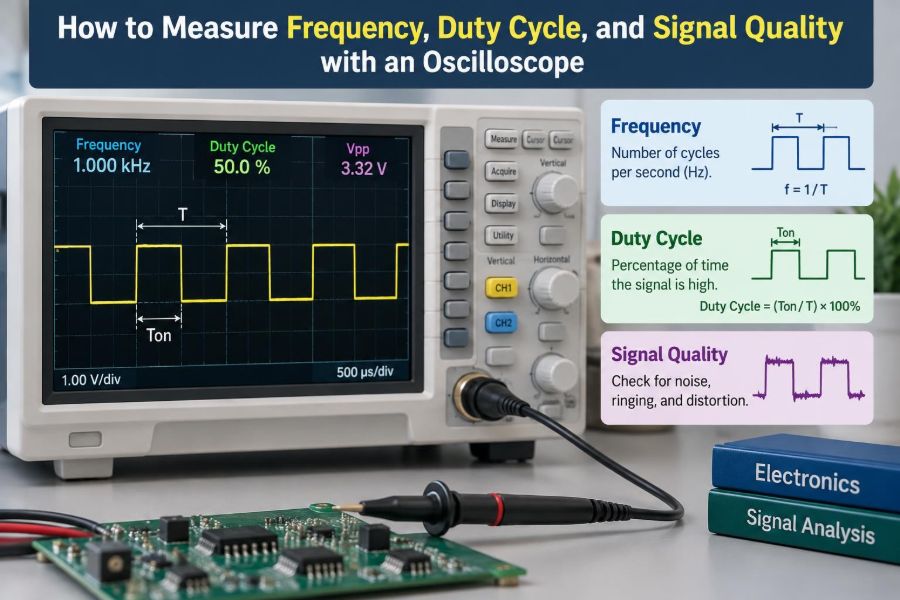
A periodic waveform repeats after a time called its period, written as T. Frequency, written as f, is the number of repetitions per second:
f = 1 / TIf one complete cycle takes 2 ms, the frequency is 500 Hz. If it takes 20 ns, the frequency is 50 MHz. Measure between equivalent points on adjacent cycles, such as rising edge to rising edge, rather than between arbitrary crossings.
⏱️ Define Duty Cycle Correctly
Duty cycle is the fraction of one period spent in the active state, usually the high state for a conventional positive-going digital signal:
Duty cycle (%) = (high time / period) × 100A 10 kHz PWM waveform has a 100 µs period. If it remains high for 25 µs, its duty cycle is 25%. Some systems define “active” as low, especially with signals named /CS or /RESET; always identify the intended active polarity.
🛠️ Choose the Right Probe First
A standard passive 10× probe is the usual starting point for general electronic work. It reduces the voltage reaching the scope input by a factor of ten and, in many cases, presents less capacitance to the circuit than a 1× probe.
That lower capacitance matters on fast or high-impedance nodes. A 1× probe can visibly slow an edge or distort a small timing capacitor waveform. Set the probe factor correctly both on the probe body and in the oscilloscope channel menu, or every displayed voltage measurement will be wrong.
⚠️ Understand the Ground Clip Hazard
On many bench oscilloscopes, the probe ground clip is connected to protective earth through the scope power cord. It is not a floating reference lead. Clipping it to a non-ground point can create a short circuit through earth.
For mains-referenced power electronics, use an appropriate isolated differential probe, a properly designed isolated measurement arrangement, or professional guidance. Never defeat protective grounding with an unsafe adapter simply to make a measurement convenient.
🎛️ Compensate the Passive Probe
Connect a passive probe to the scope’s calibration output and adjust its compensation trimmer as specified by the probe manufacturer. The displayed square wave should have a flat top and clean corners.
- Undercompensation rounds the edges and can make rise time appear slower.
- Overcompensation produces a peaked or distorted edge.
- Correct compensation gives the probe a suitably flat response for that scope input.
This adjustment does not make every measurement perfect, but it removes a basic source of probe-induced error.
🧷 Connect at the Point That Matters
Measure at the receiver when investigating whether a signal is being interpreted correctly. A clean waveform at a microcontroller pin does not prove that the same waveform is clean at the far end of a cable or at a gate-driver input.
For power-stage diagnosis, the relevant point might be directly across a switching device, a current-sense resistor, or the output capacitor. The question being asked should determine both the probe location and its reference point.
🪝 Use a Short Ground Connection for Fast Edges
The long alligator ground lead supplied with a probe forms a loop with the probe tip. At fast edge rates, that loop picks up magnetic interference and adds inductance, often creating ringing that is mostly a measurement artifact.
Use a ground spring or a very short ground connection when probing high-speed digital edges and switch nodes. If the apparent oscillation shrinks dramatically with a shorter return path, treat the original trace with skepticism.
🎯 Stabilize the Display with Triggering
Triggering tells the oscilloscope when to begin drawing or capturing a waveform. For a repeating pulse train, select edge trigger, choose the measured channel, and trigger on the rising or falling edge that is relevant to the circuit.
Set the trigger level between the valid low and high levels. A trigger level placed near noise or a slowly moving threshold can make the display jump, while a stable trigger makes period and width measurements meaningful.
🔍 Set Timebase and Vertical Scale
Display several cycles when checking frequency so that irregularity is visible, then zoom into one or two cycles when measuring pulse width or edge behavior. Too many cycles make small timing features difficult to resolve; too few hide variation.
Adjust vertical scale so the signal occupies a useful portion of the screen without clipping. Clipping removes information about overshoot, while an excessively small waveform makes noise and cursor placement harder to judge.
🧮 Measure Frequency with Cursors
Time cursors provide a transparent manual method. Place one cursor on a defined feature of one cycle and the second on the equivalent feature of the next cycle. The cursor difference is the period; calculate frequency using f = 1/T.
For example, a measured interval of 4.00 µs corresponds to 250 kHz. Cursors are especially useful when automatic measurements are confused by noise, unusual waveform shape, missing pulses, or multiple transitions.
🤖 Use Automatic Frequency Measurements Wisely
Most digital scopes can calculate frequency, period, positive width, negative width, and duty cycle automatically. These functions are fast and convenient, particularly for stable signals with clear logic-like transitions.
Do not accept the number without checking what the scope selected. A noisy trace may cross the threshold several times, and a burst waveform may not have a single meaningful frequency. Compare the reported value with the visible period and the expected circuit behavior.
📏 Measure Duty Cycle from Pulse Width
Use automatic positive-width and period measurements, or use cursors to find both values. Divide high time by period, then multiply by 100. The same method works for negative duty cycle when low time is the active interval.
A useful check is that high time plus low time should equal one period for a conventional continuous waveform. If it does not, investigate measurement thresholds, glitches, missing portions of the acquisition, or an incorrect interpretation of the waveform.
🧠 Know Which Threshold Defines “High”
Pulse width is not an absolute geometric property of a sloped edge. It depends on a threshold. Oscilloscopes often use percentage thresholds between the top and base levels, while a digital receiver has actual input thresholds determined by its technology and supply conditions.
For slow edges, the difference matters. A 3.3 V signal transitioning slowly through a receiver’s threshold region can create uncertain timing even if the scope’s 50% duty-cycle measurement looks symmetrical.
🌊 Recognize Analog Waveforms and Zero Crossings
For sine waves, frequency is commonly measured from one positive-going zero crossing to the next, or from peak to peak. Duty cycle is generally not the primary description because a sine wave does not have discrete high and low states.
When a comparator converts a sine wave into a square wave, its duty cycle can reveal threshold offset. A shifted threshold causes the output to spend longer in one state, even when the input frequency remains unchanged.
⚙️ Interpret PWM Beyond Its Percentage
Pulse-width modulation controls average energy by varying on-time, but the details matter. In a motor controller, duty cycle affects average applied voltage; in a switching regulator, it relates to conversion behavior but is also influenced by topology and operating mode.
Check frequency and duty cycle together. A hypothetical 40% PWM signal at 20 kHz behaves very differently from 40% at 200 Hz when driving a motor, LED, heater, or filter, because the load and control loop respond over time.
📊 Use Persistence to Find Intermittent Behavior
Persistence keeps previous acquisitions visible, building a density-like view of where the trace occurs. A perfectly repetitive edge remains narrow; timing variation spreads the edge horizontally; amplitude variation spreads it vertically.
This is valuable for spotting intermittent jitter, occasional overshoot, or a sporadic extra pulse. Persistence reveals patterns, but it does not identify the cause by itself; correlate the event with enable signals, load changes, or other channels.
🪜 Evaluate Rise Time and Fall Time
Rise time and fall time describe how quickly a signal transitions. Scopes commonly measure between 10% and 90% of the amplitude range, avoiding the less stable extremes near the top and bottom.
Slow edges reduce timing margin and can increase switching losses in power devices. Very fast edges improve timing but can increase electromagnetic interference, transmission-line reflections, and ground-bounce sensitivity. Faster is not automatically better.
📡 Look for Overshoot, Undershoot, and Ringing
Overshoot rises beyond the intended final level; undershoot falls below the intended lower level; ringing is a decaying oscillation after a transition. These effects can result from trace inductance, impedance mismatch, package parasitics, poor decoupling, or the probe’s own ground loop.
Evaluate their magnitude, duration, and location. A brief small overshoot may be harmless in one circuit, while an excursion beyond an IC’s permitted input range can cause reliability concerns or incorrect behavior in another.
🧱 Distinguish Real Ringing from Probe Artifacts
Change one measurement condition at a time. First shorten the ground return, then compare a second probe or a different probing method, and finally inspect the same node at another physical location.
If the waveform changes greatly when the probe arrangement changes, the setup is participating in the measurement. This does not prove that the circuit is clean, but it prevents designing a “fix” for an artifact.
📉 Measure Noise with Appropriate Bandwidth
Every measurement includes some noise from the circuit, probe, scope front end, and surrounding environment. A bandwidth-limit function can reduce high-frequency displayed noise and make low-frequency ripple easier to quantify.
Use the bandwidth that matches the question. Limiting bandwidth is reasonable when assessing low-frequency power-rail ripple, but it can hide fast switching spikes that matter for an absolute-maximum rating or EMC investigation.
🧪 Check Supply Ripple at the Load
Power-rail quality is measured where the load consumes power, not only at the regulator output. Use short probing connections across the local decoupling capacitor and select AC coupling if a small ripple must be viewed on top of a large DC rail.
AC coupling removes the displayed DC component but does not make the underlying rail safer or cleaner. Record the coupling mode, bandwidth limit, probe factor, and load condition so the measurement can be reproduced.
🧩 Watch for Glitches and Missing Pulses
A narrow glitch may be too brief to notice in a normal rolling display, yet it can clock a flip-flop, reset a peripheral, or trigger an interrupt. Use single acquisition, glitch trigger, pulse-width trigger, or a long record length depending on what the scope provides.
For a control signal expected to remain high, configure a trigger for a pulse shorter than the expected duration. This lets the oscilloscope capture the exception rather than repeatedly showing the normal state.
🗂️ Choose Sample Rate and Memory Depth
Sample rate determines how frequently the scope records points; memory depth determines how long it can record at useful detail. A long time window may force the instrument to lower its sample rate unless sufficient memory is available.
Undersampling can hide glitches or create misleading alias patterns. As a practical habit, zoom into the acquired record and confirm that transitions contain enough points to support the conclusion. For demanding high-frequency work, consult the scope’s bandwidth and sampling specifications rather than relying on appearance alone.
🔄 Avoid Aliasing and Display Deception
Aliasing occurs when sampling cannot adequately represent the waveform’s changing content. A fast repetitive signal may appear as a slower waveform, drift across the screen, or show an invented low-frequency pattern.
Change the timebase and observe whether the displayed frequency remains physically plausible. When possible, use a faster sample rate, reduce the time span, or use acquisition modes designed for repetitive signals. A stable-looking trace is not necessarily a truthful trace.
🧷 Use AC and DC Coupling Deliberately
DC coupling displays both DC level and changing components, making it the default for logic-level verification and absolute voltage checks. AC coupling blocks the DC component at the input and helps magnify ripple or small variations.
AC coupling changes the low-frequency response, so it can distort very slow signals and long pulses. Do not use it when accurate DC level, duty cycle of slow pulses, or baseline behavior is the question.
🧰 Compare Measurement Methods
| Method | Best use | Main limitation |
|---|---|---|
| Grid estimate | Fast plausibility check | Limited precision |
| Time cursors | Unusual or noisy waveforms | Depends on cursor placement |
| Automatic measurements | Stable repetitive signals | Can misread glitches or thresholds |
| Frequency counter function | Precise stable repetition rate | May not reveal waveform defects |
The strongest practice is to use two methods when the result affects a design decision. A frequency number that agrees with visible period spacing is more credible than either observation alone.
🧱 Account for Loading and Bandwidth
A probe and scope are part of the circuit during measurement. Probe resistance, capacitance, input capacitance, and bandwidth can alter what is observed, especially in high-impedance, high-frequency, or high-voltage circuits.
Scope bandwidth also limits observed edge speed. A measured rise time includes both the signal and instrument response; therefore, do not claim a source edge is faster than the instrument can resolve. Use a probe and scope rated appropriately for the signal’s voltage, frequency content, and energy.
🧾 Document Conditions, Not Just Numbers
A useful measurement note includes the probe type and attenuation, channel coupling, bandwidth limit, timebase, triggering method, test point, load state, and relevant circuit configuration. A screenshot without these conditions can be difficult to interpret later.
For a PWM test, state whether the load was connected, whether the controller was in startup or steady state, and where ground was attached. This turns a one-time observation into engineering evidence another person can repeat.
🚫 Avoid Common Measurement Mistakes
- Reading frequency from a display that is not stably triggered.
- Trusting automatic duty cycle on a waveform with ringing near its threshold.
- Using a long ground lead for a fast switching node.
- Measuring a remote load’s supply quality at the regulator instead of at the load.
- Ignoring probe attenuation settings or probe compensation.
- Assuming a clean periodic display rules out rare glitches.
- Connecting an earth-referenced probe ground to a hazardous non-ground node.
Most of these errors produce believable waveforms. That is why a deliberate setup matters more than simply obtaining a stable trace.
✅ Build a Repeatable Measurement Routine
- Identify the signal’s expected voltage range, frequency range, reference, and safety risks.
- Select a suitable probe and verify attenuation and compensation.
- Connect with the shortest practical ground return.
- Set DC coupling first, appropriate vertical scale, and a timebase showing several cycles.
- Establish a stable trigger at a meaningful threshold.
- Check period manually, then use automatic frequency and width measurements.
- Zoom into edges and inspect for ringing, glitches, noise, and timing variation.
- Record the setup and repeat under relevant load or operating conditions.
🏁 Make the Waveform Answer the Engineering Question
A useful oscilloscope measurement is not merely a number on screen. It links an observed waveform to a circuit requirement: a clock meets timing, a PWM output delivers intended control, a rail remains within acceptable behavior, or a data line reaches valid logic levels with sufficient margin.
Frequency describes repetition, duty cycle describes time allocation, and signal quality describes whether real hardware can tolerate the waveform’s amplitude, edges, noise, and exceptions. Treat all three as parts of the same diagnosis.
The best oscilloscope measurements combine correct probing, sensible triggering, independent checks, and an understanding of what the receiving circuit actually needs. Once those habits become routine, a waveform stops being a picture and becomes evidence. 🔌📈🛠️