
A thermostat decides whether to run a heater. A smartwatch estimates a pulse. A drone holds its altitude while moving through gusty air. None of these systems begins with neat numbers; each begins with a physical quantity that changes continuously.
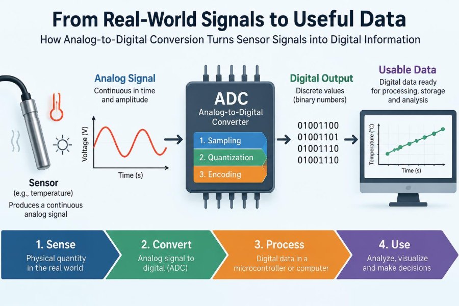
Temperature, light, pressure, sound, acceleration, and voltage are analog phenomena. A microcontroller, however, stores, compares, transmits, and acts on numbers. The bridge between those two domains is analog-to-digital conversion, usually shortened to ADC.
It is tempting to view an ADC as a small peripheral that simply “reads a voltage.” That view hides the engineering decisions that determine whether a reading is stable, accurate, timely, and meaningful—or merely a convincing-looking wrong number.
Understanding the full signal path helps when selecting a sensor, debugging noisy measurements, choosing a sampling rate, or interpreting a value from a datasheet. The conversion itself matters, but so does everything that happens before and after it.
🌍 Physical quantities are inherently analog
An analog quantity can take any value within a continuous range. The air temperature might move gradually from 21.1°C to 21.12°C, and microphone voltage follows the changing pressure of a sound wave without stepping through integer levels.
Sensors respond to a physical input and produce an electrical effect: often voltage, current, resistance, capacitance, charge, or frequency. A thermistor changes resistance with temperature, a photodiode produces current from light, and a strain gauge changes resistance when stretched.
The rest of an electronic system needs a representation it can process repeatedly and reliably. That representation is a finite set of binary numbers.
🔢 Digital data is a deliberately limited representation
A digital value is not the physical world itself. It is a coded measurement made at a particular moment, with limited amplitude detail. An 8-bit converter has 256 possible output codes; a 12-bit converter has 4,096.
That finite code range is useful because digital circuitry can store values in memory, run control algorithms, display trends, trigger alarms, and send data over a network. It is also repeatable: the same valid code means the same numerical value wherever it is processed.
The trade-off is unavoidable. Conversion replaces a continuous signal with discrete values in both time and amplitude.
🧭 The complete sensor-to-data signal chain
An ADC is one stage in a measurement chain, not a universal accuracy device. A typical path is:
- A physical quantity affects a sensor.
- The sensor creates an electrical signal.
- Analog circuitry protects, powers, filters, and scales that signal.
- The ADC samples and quantizes it into a code.
- Firmware calibrates, filters, interprets, and uses the code.
An error introduced near the sensor cannot generally be repaired by a higher-resolution ADC. For example, a poorly mounted temperature sensor may faithfully report the temperature of a nearby hot circuit rather than the intended air.
⚡ Sensors do not all produce ADC-ready voltages
Some sensors have a voltage output designed to connect directly to an ADC input. Others need excitation or conversion circuitry. A resistive sensor may be placed in a voltage divider, while a photodiode commonly needs a transimpedance amplifier to turn its current into voltage.
Many modern sensor modules contain their own amplifier, ADC, calibration memory, and digital interface such as I²C or SPI. In that case, the ADC still exists, but it is inside the module rather than inside the host microcontroller.
Choosing the interface should follow the measurement need. An integrated digital sensor reduces analog design work, while a raw analog sensor can offer flexibility when the signal chain must be tailored carefully.
📏 Voltage range defines what the ADC can see
An ADC compares its input voltage with a reference range. In an ideal unipolar converter with a 0 V lower limit and reference voltage VREF, inputs from 0 V to VREF map to output codes from zero to the maximum code.
Inputs below the lower limit or above the upper limit cannot be represented correctly. They usually produce an endpoint code, known as clipping or saturation. A clipped waveform loses information even if its digital output appears stable.
Signal conditioning should keep the expected signal in range, including normal variation, tolerances, and transients. Leaving a small design margin is often wiser than mapping an uncertain maximum exactly to full scale.
🎚️ Reference voltage sets the measuring ruler
The reference voltage is the ADC’s ruler. If an ideal 12-bit ADC uses a 3.3 V reference, one nominal code step is approximately 3.3 / 4096 volts. If the reference changes, the voltage represented by each code changes too.
A supply rail can serve as a reference in simple ratiometric systems, especially where both the sensor output and ADC reference scale with the same supply. A potentiometer powered by that rail is a familiar example: its position ratio remains approximately the same even when the supply moves slightly.
For an absolute voltage measurement, the reference needs suitable accuracy, noise performance, temperature behavior, and layout. A precise ADC paired with an unstable reference is not a precise measurement system.
🪜 Resolution describes code spacing, not guaranteed accuracy
Resolution tells us how many output levels are available. For an ideal N-bit ADC, there are 2^N possible codes. The nominal least significant bit, or LSB, is the full-scale range divided by that number of levels.
More bits create finer code spacing, but they do not automatically reveal smaller real-world changes. Sensor noise, reference noise, offset, nonlinearity, and interference can make the bottom bits fluctuate or become inaccurate.
For example, moving from 10 bits to 12 bits reduces nominal code width by a factor of four. That can be valuable only when the analog signal chain and measurement conditions are quiet and stable enough to use it.
🧮 Quantization turns a continuum into steps
During quantization, each sampled input is assigned to the nearest—or, depending on architecture, a defined—digital code. The original voltage can no longer be known exactly from that code; only an interval associated with the code is known.
The resulting difference is quantization error. In an ideal converter, it is bounded roughly within half of one LSB under common rounding conventions. It is not necessarily random in every real signal, but it establishes a fundamental limit on amplitude granularity.
A slowly changing input therefore produces a staircase-shaped sequence of codes. This is expected behavior, not automatically a fault.
📸 Sampling captures voltage at specific instants
Sampling answers a different question from resolution: not “how finely is voltage divided?” but “when is the voltage observed?” The ADC measures the signal at discrete times separated by the sampling period.
Many ADCs use a sample-and-hold circuit. A small internal capacitor briefly connects to the input, acquires its voltage, then holds that voltage while the converter determines the code.
This mechanism has practical consequences. If the source cannot charge that internal capacitor quickly enough, the recorded voltage may be wrong, particularly at short acquisition times or with high source impedance.
🎵 Sampling rate must match signal bandwidth
The sampling rate is the number of samples taken per second. To represent a band-limited signal without frequency overlap, the sampling rate must exceed twice the highest frequency component of interest. This is the core idea behind the Nyquist sampling criterion.
In practice, sampling only slightly above twice the desired bandwidth makes filter design difficult. Engineers usually provide margin because real filters do not switch from passband to complete rejection at one perfectly sharp frequency.
A room-temperature monitor may need only occasional readings. Audio, vibration, motor current ripple, and rapidly changing control loops may need far higher rates. Faster is not always better: it increases processing, power use, storage, and sensitivity to design limitations.
🌀 Aliasing creates false low-frequency information
When frequencies above half the sampling rate reach the ADC, they can appear in the data as lower, incorrect frequencies. This is called aliasing. Once it has occurred, software cannot reliably determine which part of the recorded pattern was real and which part was folded from a higher frequency.
A useful analogy is a video of a rotating wheel that appears to slow down or rotate backward. The wheel has not changed direction; the camera sampled it too slowly to represent its motion unambiguously.
Before conversion, use an analog low-pass filter to attenuate unwanted high-frequency energy. This anti-alias filter should be selected alongside the sample rate, not as an afterthought.
🧰 Signal conditioning prepares the input
Signal conditioning is the analog work between sensor and ADC. It may include amplification, attenuation, level shifting, filtering, buffering, sensor excitation, isolation, and input protection.
A bridge-based pressure sensor might generate a very small differential voltage. An instrumentation amplifier can amplify the difference while rejecting voltage common to both leads, then shift the result into the ADC’s allowed input range.
Conditioning is not about making every signal large. It is about making the signal compatible with the ADC without distorting the information that matters.
📈 Gain uses available codes more effectively
If a 0 to 100 mV sensor signal enters a 0 to 3.3 V ADC without amplification, it uses only a small portion of the converter’s code range. The nominal voltage spacing at the input is then much larger relative to the sensor signal than necessary.
Appropriate gain can expand that signal toward full scale and improve usable detail. Yet excessive gain is risky: sensor offset, drift, unexpected conditions, and amplifier noise can drive the input into saturation.
Design from the complete expected range, not only the ideal nominal output. Include sensor tolerance, supply variation, temperature effects, and fault behavior where relevant.
↔️ Differential inputs reject shared disturbances
A single-ended ADC measures a signal relative to a shared ground. A differential ADC measures the difference between two input nodes. Differential measurement can reduce sensitivity to disturbances that appear similarly on both wires, such as some ground shifts or coupled noise.
This is especially useful with bridge sensors, long sensor leads, and small signals. It is not magic noise removal: the ADC and front end have limits on allowed common-mode voltage, input range, and common-mode rejection.
Twisted-pair wiring, sensible cable routing, and a suitable amplifier often complement differential conversion better than relying on the ADC input configuration alone.
🧪 ADC architectures make different trade-offs
Different converter architectures optimize for different combinations of speed, resolution, power, latency, and cost. The “best ADC” depends on the signal and application.
| Architecture | Typical strength | Common use |
|---|---|---|
| SAR | Good balance of speed, power, and resolution | Microcontrollers, control systems, data acquisition |
| Sigma-delta | High resolution for low-bandwidth signals | Weigh scales, precision sensors, audio |
| Flash | Very high conversion speed | High-speed communications and instruments |
| Pipeline | High throughput at moderate-to-high resolution | Imaging, RF-related and fast acquisition systems |
SAR, or successive-approximation-register, converters are common in embedded devices. Sigma-delta converters use oversampling and digital filtering, but their filters can add latency that matters in fast control applications.
🔍 What a SAR ADC does during conversion
A SAR ADC performs a binary search. After sampling the input, it first tests whether the input is above or below half-scale. It retains or clears the most significant bit, then tests the next bit, repeating until it has built the final code.
Internally, this process uses a comparator and a digital-to-analog converter, often a capacitor array. Each decision narrows the remaining voltage interval, much like repeatedly halving the range in a number-guessing game.
This approach is efficient and predictable, but it requires adequate acquisition time, a stable reference, and an input signal that does not violate converter timing requirements.
⏱️ Conversion time, throughput, and latency differ
Conversion time is how long the ADC needs to turn a held sample into a code. Throughput is how many conversions can be completed per second. Latency is the delay between an input event and availability of a usable output.
These terms are related but not interchangeable. A sigma-delta ADC may output samples at a stated data rate while its digital filter creates delay. A multiplexed ADC may have high total throughput but lower effective rate per channel.
For a protection system or closed-loop controller, delayed data can be as problematic as inaccurate data. Read timing diagrams and filter settings, not just the headline samples-per-second figure.
🧷 Source impedance affects sampling accuracy
The sample-and-hold capacitor draws a brief charging current when it connects to the input. A high-resistance source, such as a large-value voltage divider or some unbuffered sensor circuits, may not settle to the correct voltage during acquisition.
The error can vary with the previous channel’s voltage, making it seem mysterious. Switching from a high-voltage channel to a high-impedance low-voltage channel may leave residual charge that biases the next reading.
Possible remedies include a longer acquisition time, lower resistor values where power permits, a buffer amplifier, a small input capacitor used carefully, or a dummy conversion after channel switching.
🔀 Multiplexing channels introduces settling concerns
Many microcontroller ADCs share one converter among several input channels through an analog multiplexer. This saves silicon area and cost, but changing channels does not instantly erase the electrical history of the sampling network.
Channels with different voltage levels or source impedances need time to settle. Reading a high-impedance sensor immediately after a rapidly changing high-level signal can produce a biased first result.
Group similar channels when possible, configure individual sample times if supported, and verify the behavior with known test voltages. Discarding a first reading can help, but it should be a measured design choice rather than a ritual.
🌩️ Noise enters through more paths than expected
Noise may originate in the sensor, amplifier, reference, supply rails, digital switching currents, electromagnetic coupling, or the environment. A long lead near a motor drive can pick up interference even when the ADC itself is functioning correctly.
Random noise causes code jitter. Periodic interference may create repeating patterns tied to switching regulators, mains coupling, displays, or communication bursts. Looking at raw samples over time is often more revealing than inspecting only an average.
Ground routing, shielding, decoupling, controlled return paths, filtering, and physical separation all matter. There is no single “noise fix” because the source and coupling path determine the effective remedy.
🧱 Grounding and layout are part of the measurement circuit
An ADC measures voltage differences, so ground is not an abstract zero-voltage symbol. Current flowing through a ground trace creates a voltage drop. If digital return current shares part of the path used as an analog reference, switching activity can appear directly in measurements.
Keep sensitive analog routes short, place reference and supply decoupling capacitors close to the relevant pins, and follow the device manufacturer’s layout guidance. Separate noisy power loops from small sensor signals.
“Split analog and digital ground” is not a universal rule. The goal is to manage return-current paths and avoid forcing noisy currents through sensitive measurement references. Board stack-up, frequency, converter type, and layout all influence the correct approach.
🛡️ Protecting an ADC input needs restraint
Real inputs can experience ESD, cable transients, wrong connections, and voltages when the ADC supply is off. Protection may use series resistance, external clamp diodes, transient suppressors, fuses, or dedicated protection devices.
Every protection component has electrical consequences. Excess series resistance can worsen acquisition settling; clamp leakage can distort tiny signals; capacitance can limit bandwidth. Internal protection diodes also have current limits and should not be assumed to absorb unlimited fault energy.
Design protection around credible fault conditions and consult the ADC or microcontroller absolute-maximum ratings. A circuit that survives a laboratory bench test may still be unsuitable for an exposed industrial cable.
🧹 Digital filtering improves usability, with trade-offs
After conversion, firmware can reduce random variation or remove selected frequency components. A moving average smooths noise but responds more slowly to real changes. A median filter can reject occasional spikes, while a low-pass IIR filter uses little memory but introduces phase delay.
The right filter follows the meaning of the measurement. A tank-level display can be deliberately calm; a collision detector must respond quickly. Filtering an alarm signal too aggressively can hide the very event the system must detect.
Always inspect both raw and filtered data during development. A smooth graph is not proof of a correct measurement—it may simply be proof of a strong filter.
➕ Oversampling can help, but it cannot create truth
Taking multiple samples and averaging can reduce uncorrelated random noise. Oversampling followed by averaging or decimation can also improve effective resolution when the signal includes enough natural or introduced dither to move among adjacent codes.
It cannot recover information lost to clipping, correct gain error, remove a coherent interference tone reliably, or compensate for a sensor that is inaccurate. Repeating the same biased measurement only produces a more stable biased result.
Use oversampling after verifying bandwidth and timing. The aggregate sampling rate must still be high enough, and the averaging window must not conceal changes that matter.
🎯 Accuracy includes several separate error sources
Resolution is only one specification. A practical error budget may include sensor accuracy, sensor nonlinearity, amplifier offset and gain error, reference error, ADC offset, ADC gain error, integral nonlinearity, noise, and temperature drift.
Offset error shifts readings by a nearly constant amount. Gain error changes the scale. Integral nonlinearity, often abbreviated INL, describes departure from an ideal straight transfer curve. These errors affect measurements differently and need different correction approaches.
Do not add every datasheet maximum blindly without understanding whether terms are independent, calibrated, or specified under different conditions. An error budget is a model of a particular system and operating range.
🧭 Calibration connects codes to real units
An ADC output code initially represents an electrical input, not necessarily temperature, pressure, force, or concentration. Calibration establishes the relationship between measured code and a known physical quantity.
A simple one-point calibration removes an offset. Two-point calibration can correct offset and slope over a limited range. More complex sensors may need lookup tables, polynomial correction, or piecewise linear interpolation to account for nonlinearity.
Calibration is valid only under stated conditions and over time scales appropriate to the device. Mechanical stress, aging, temperature, and sensor replacement can change the relationship. Record calibration assumptions rather than treating a coefficient as timeless.
🌡️ Temperature and time cause drift
Components change with temperature. Sensor sensitivity, resistor values, amplifier offset, reference voltage, and ADC behavior can all move. A reading that is excellent on a bench at one temperature may shift in an enclosure, outdoors, or beside a power stage.
Time introduces additional changes through aging, contamination, mechanical relaxation, and battery behavior. The seriousness depends on the required measurement uncertainty and the application’s consequences.
Good designs identify dominant drift sources early. Sometimes periodic calibration is appropriate; in other cases, selecting a better reference, using ratiometric measurement, or measuring local temperature for compensation is more effective.
🧠 Firmware must preserve measurement meaning
Firmware should label units, ranges, timestamps, fault states, and calibration versions clearly. Storing a raw code is useful for diagnostics, but a control decision should not confuse “ADC count” with a physically calibrated quantity.
Use suitable integer widths and check arithmetic scaling. A common error is overflow while multiplying ADC counts before division. Fixed-point arithmetic can be efficient and deterministic, provided its scale and rounding behavior are defined.
Also detect implausible values: endpoint codes, disconnected sensors, stale data, and abrupt steps beyond credible physical behavior may deserve separate handling rather than being silently displayed as normal readings.
🔧 A practical workflow for designing a measurement channel
Start from the physical question, not the ADC catalog page. Ask what must be measured, how fast it changes, what uncertainty is acceptable, and what environmental or safety conditions apply.
- Determine the sensor’s output type, range, impedance, bandwidth, and excitation needs.
- Define input scaling, reference choice, protection, and required analog filtering.
- Select ADC range, resolution, architecture, sampling rate, and channel timing.
- Estimate the main errors and noise sources across operating conditions.
- Plan calibration, diagnostics, firmware filtering, and validation tests.
Then test the chain as a chain. Inject known electrical inputs, compare with trusted instruments where appropriate, observe raw codes, vary temperature or load when practical, and verify behavior at range limits.
🚫 Common ADC mistakes and better alternatives
Several shortcuts repeatedly produce misleading results:
- Mistake: treating bit count as accuracy. Better: assess reference, noise, linearity, sensor error, and layout.
- Mistake: sampling a noisy signal faster without anti-alias filtering. Better: define bandwidth first, then filter and sample accordingly.
- Mistake: driving an ADC from a high-impedance divider without checking acquisition time. Better: calculate or measure settling and add a buffer or timing margin.
- Mistake: averaging away a recurring fault pattern. Better: identify periodic interference at its source.
- Mistake: calibrating only at room conditions. Better: evaluate the operating range that matters.
🏭 The right design depends on the application
A battery monitor may prioritize low quiescent current and tolerate a slow reading. An audio recorder needs adequate bandwidth, low distortion, and carefully controlled sampling. A laboratory instrument may favor traceability and thermal stability over low cost.
In a motor controller, measurements must arrive quickly enough for stable control and survive electrical noise. In a medical or safety-related device, requirements may also include fault detection, isolation, verification, and applicable regulatory processes beyond ordinary measurement performance.
There is no isolated ADC specification that solves every use case. The appropriate design is the one whose complete measurement chain supports the required decision.
🧩 The core principle: conversion is a system task
Analog-to-digital conversion gives software access to the electrical evidence produced by a sensor. It samples that evidence in time, maps it into finite codes, and makes it available for computation.
But trustworthy data depends on more than the conversion step. The sensor must represent the intended physical quantity, the front end must preserve and scale the signal, the reference and layout must be stable, sampling must respect bandwidth, and firmware must interpret limitations honestly.
When a measurement seems wrong, trace the signal from physical stimulus to final number. That disciplined approach is usually more productive than changing the ADC setting at random.
Useful digital data begins with a well-designed analog measurement path, not merely a high-resolution converter. Once that principle guides the design, sensors become dependable sources of information rather than mysterious streams of fluctuating counts. 🔌📊🛠️